1. Two analysis steps were defined: a static step to apply internal pressure, and a transient step to analyze creep over 50 years.
2. Output requests were specified to write displacements, stresses, and creep strains to the output database every 2 increments, as well as displacements at a point.
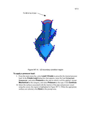
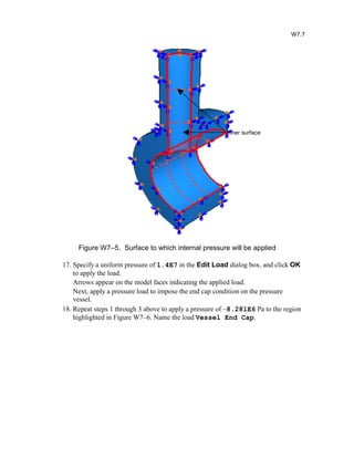
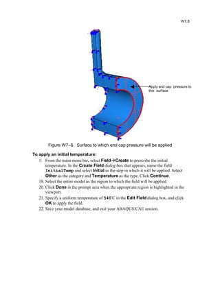
3. Boundary conditions of symmetry and a displacement constraint were applied, and internal pressure and end cap pressure loads were prescribed. An initial temperature of 540°C was also specified.
![10. From the main menu bar, select BCCreate to prescribe boundary conditions
on the model. In the Create Boundary Condition dialog box that appears,
name the boundary condition X-SYMM and select Initial as the step in which it
will be applied. Accept Mechanical as the category and Symmetry/
Antisymmetry/Encastre as the type. Click Continue.
You may need to rotate the view to facilitate your selection in the following steps.
11. Select ViewRotate from the main menu bar (or use the tool from the
toolbar), and drag the cursor over the virtual trackball in the viewport. The view
rotates interactively; try dragging the cursor inside and outside the virtual
trackball to see the difference in behavior.
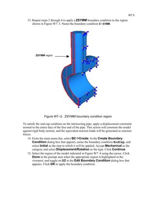
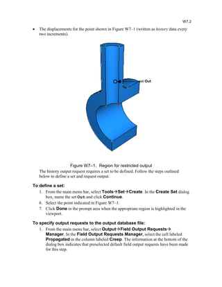
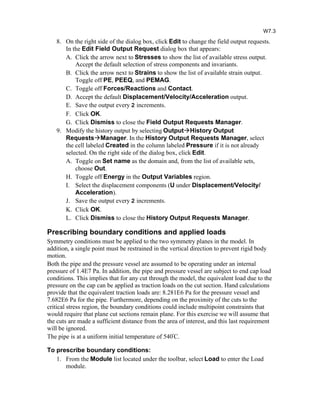
12. Select the regions of the model indicated in Figure W7–2 using [Shift]+Click.
Click Done in the prompt area when the appropriate regions are highlighted in
the viewport, and toggle on XSYMM in the Edit Boundary Condition dialog
box that appears. Click OK to apply the boundary condition.
Figure W7–2. XSYMM boundary condition region
Arrows appear on the face indicating the constrained degrees of freedom. The
XSYMM boundary condition constrains the degrees of freedom necessary to
impose symmetry about a plane X = constant; after the part is meshed and the job
is created, this constraint will be applied to all the nodes that occupy the region.
W7.4
XSYMM regions](https://image.slidesharecdn.com/workshop7-creep-steps-130825051329-phpapp01/85/Workshop7-creep-steps-4-320.jpg)