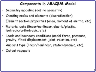
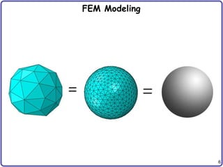
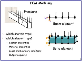
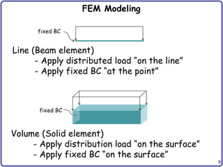
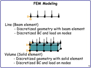
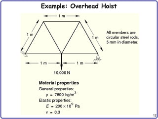
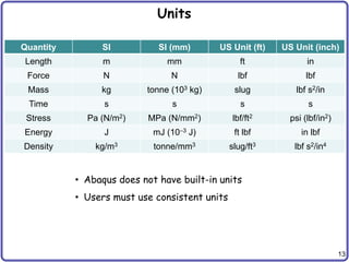
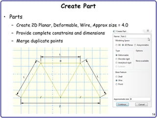
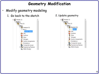
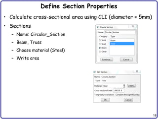
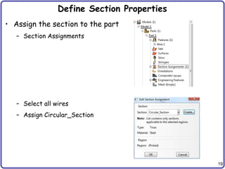
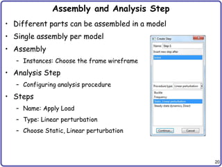
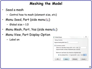
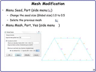
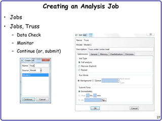
1
Finite Element Analysis
Using Abaqus
2
Abaqus Basics
Simulation
Abaqus/Standard
Output file:
Job.odb, job.dat
Postprocessing
Abaqus/CAE
Preprocessing
Abaqus/CAE
Interactive Mode
Analysis Input file
Input file (text):
Job.inp
FEM Solver
3
Methods of Analysis in ABAQUS
• Interactive mode
– Create an FE model and analysis using GUI
– Advantage: Automatic discretization and no need to remember
commands
– Disadvantage: No automatic procedures for changing model or
parameters
• Python script
– All GUI user actions will be saved as Python script
– Advantage: Users can repeat the same command procedure
– Disadvantage: Need to learn Python script language
4
Methods of Analysis in ABAQUS
• Analysis input file
– ABAQUS solver reads an analysis input file
– Possible to manually create an analysis input file
– Advantage: Users can change model directly without GUI
– Disadvantage: Users have to discretize model and learn ABAQUS
input file grammar
5
Components in ABAQUS Model
• Geometry modeling (define geometry)
• Creating nodes and elements (discretization)
• Element section properties (area, moment of inertia, etc)
• Material data (linear/nonlinear, elastic/plastic,
isotropic/orthotropic, etc)
• Loads and boundary conditions (nodal force, pressure,
gravity, fixed displacement, joint, relation, etc)
• Analysis type (linear/nonlinear, static/dynamic, etc)
• Output requests
6
FEM Modeling
7
FEM Modeling
Pressure
• Which analysis type?
• Which element type?
– Section properties
– Material properties
– Loads and boundary conditions
– Output requests
Beam element
Solid element
8
Line (Beam element)
- Assign section properties (area, moment
of inertia)
- Assign material properties
Volume (Solid element)
- Assign section properties
- Assign material properties
FEM Modeling
9
FEM Modeling
Line (Beam element)
- Apply distributed load “on the line”
- Apply fixed BC “at the point”
Volume (Solid element)
- Apply distribution load “on the surface”
- Apply fixed BC “on the surface”
fixed BC
fixed BC
10
FEM Modeling
Line (Beam element)
- Discretized geometry with beam element
- Discretized BC and load on nodes
Volume (Solid element)
- Discretized geometry with solid element
- Discretized BC and load on nodes
11
Start Abaqus/CAE
• Startup window
12
Example: Overhead Hoist
13
Units
Quantity SI SI (mm) US Unit (ft) US Unit (inch)
Length m mm ft in
Force N N lbf lbf
Mass kg tonne (103 kg) slug lbf s2/in
Time s s s s
Stress Pa (N/m2) MPa (N/mm2) lbf/ft2 psi (lbf/in2)
Energy J mJ (10–3 J) ft lbf in lbf
Density kg/m3 tonne/mm3 slug/ft3 lbf s2/in4
• Abaqus does not have built-in units
• Users must use consistent units
14
Create Part
• Parts
– Create 2D Planar, Deformable, Wire, Approx size = 4.0
– Provide complete constrains and dimensions
– Merge duplicate points
15
Geometry Constraint
• Define exact geometry
– Add constraints
– Add dimension
– Over constraint warning
16
Geometry Modification
• Modify geometry modeling
1. Go back to the sketch 2. Update geometry
17
Define Material Properties
• Materials
– Name: Steel
– Mechanical
Elasticity
Elastic
18
Define Section Properties
• Calculate cross-sectional area using CLI (diameter = 5mm)
• Sections
– Name: Circular_Section
– Beam, Truss
– Choose material (Steel)
– Write area
19
Define Section Properties
• Assign the section to the part
– Section Assignments
– Select all wires
– Assign Circular_Section
20
Assembly and Analysis Step
• Different parts can be assembled in a model
• Single assembly per model
• Assembly
– Instances: Choose the frame wireframe
• Analysis Step
– Configuring analysis procedure
• Steps
– Name: Apply Load
– Type: Linear perturbation
– Choose Static, Linear perturbation
21
Assembly and Analysis Step
• Examine Field Output Request (automatically requested)
• User can change the request
22
Boundary Conditions
• Boundary conditions: Displacements or rotations are known
• BCs
– Name: Fixed
– Step: Initial
– Category: Mechanical
– Type: Displacement/Rotation
– Choose lower-left point
– Select U1 and U2
• Repeat for lower-right corner
– Fix U2 only
23
Applied Loads
• Loads
– Name: Force
– Step: Applied Load
– Category: Mechanical
– Type: Concentrated force
• Choose lower-center point
• CF2 = -10000.0
24
Meshing the Model
• Parts
– Part-1, Mesh
• Menu Mesh, Element Types (side menu )
• Select all wireframes
• Library: Standard
• Order: Linear
• Family: Truss
• T2D2: 2-node linear
2-D truss
25
Meshing the Model
• Seed a mesh
– Control how to mesh (element size, etc)
• Menu Seed, Part (side menu )
– Global size = 1.0
• Menu Mesh, Part, Yes (side menu )
• Menu View, Part Display Option
– Label on
26
Mesh Modification
• Menu Seed, Part (side menu )
– Change the seed size (Global size) 1.0 to 0.5
– Delete the previous mesh
• Menu Mesh, Part, Yes (side menu )
27
Creating an Analysis Job
• Jobs
• Jobs, Truss
– Data Check
– Monitor
– Continue (or, submit)
28
Postprocessing
• Change “Model” tab to “Results” tab
• Menu File, Open Job.odb file
• Common Plot Option (side menu ), click on the Labels tab
(Show element labels, Show node labels)
Set Font for All Model Labels…
29
Postprocessing
• Deformation scale
• Common Plot Option (side menu ), click on the Basic tab,
Deformation Scale Factor area
30
Postprocessing
• Tools, XY Data, Manager
– Position: Integration Point
– Stress components, S11 (Try
with displacements and
reaction)
31
Postprocessing
– Click on the Elements/Nodes tab
– Select Element/Nodes you want to
see result and save
– Click Edit… to see the result
32
Postprocessing
• Report, Field Output
– Position: Integration Point
– Stress components, S11 (Try
with displacements and
reaction)
– Default report file name is
“abaqus.rpt”
– The report file is generated in
“C:temp” folder
33
Save
• Save job.cae file
• Menu, File, Save As…
- job.cae file is saved
- job.jnl file is saved as well (user action history, python
code)

Abaqus Training.pptx

  • 1.
  • 2.
    2 Abaqus Basics Simulation Abaqus/Standard Output file: Job.odb,job.dat Postprocessing Abaqus/CAE Preprocessing Abaqus/CAE Interactive Mode Analysis Input file Input file (text): Job.inp FEM Solver
  • 3.
    3 Methods of Analysisin ABAQUS • Interactive mode – Create an FE model and analysis using GUI – Advantage: Automatic discretization and no need to remember commands – Disadvantage: No automatic procedures for changing model or parameters • Python script – All GUI user actions will be saved as Python script – Advantage: Users can repeat the same command procedure – Disadvantage: Need to learn Python script language
  • 4.
    4 Methods of Analysisin ABAQUS • Analysis input file – ABAQUS solver reads an analysis input file – Possible to manually create an analysis input file – Advantage: Users can change model directly without GUI – Disadvantage: Users have to discretize model and learn ABAQUS input file grammar
  • 5.
    5 Components in ABAQUSModel • Geometry modeling (define geometry) • Creating nodes and elements (discretization) • Element section properties (area, moment of inertia, etc) • Material data (linear/nonlinear, elastic/plastic, isotropic/orthotropic, etc) • Loads and boundary conditions (nodal force, pressure, gravity, fixed displacement, joint, relation, etc) • Analysis type (linear/nonlinear, static/dynamic, etc) • Output requests
  • 6.
  • 7.
    7 FEM Modeling Pressure • Whichanalysis type? • Which element type? – Section properties – Material properties – Loads and boundary conditions – Output requests Beam element Solid element
  • 8.
    8 Line (Beam element) -Assign section properties (area, moment of inertia) - Assign material properties Volume (Solid element) - Assign section properties - Assign material properties FEM Modeling
  • 9.
    9 FEM Modeling Line (Beamelement) - Apply distributed load “on the line” - Apply fixed BC “at the point” Volume (Solid element) - Apply distribution load “on the surface” - Apply fixed BC “on the surface” fixed BC fixed BC
  • 10.
    10 FEM Modeling Line (Beamelement) - Discretized geometry with beam element - Discretized BC and load on nodes Volume (Solid element) - Discretized geometry with solid element - Discretized BC and load on nodes
  • 11.
  • 12.
  • 13.
    13 Units Quantity SI SI(mm) US Unit (ft) US Unit (inch) Length m mm ft in Force N N lbf lbf Mass kg tonne (103 kg) slug lbf s2/in Time s s s s Stress Pa (N/m2) MPa (N/mm2) lbf/ft2 psi (lbf/in2) Energy J mJ (10–3 J) ft lbf in lbf Density kg/m3 tonne/mm3 slug/ft3 lbf s2/in4 • Abaqus does not have built-in units • Users must use consistent units
  • 14.
    14 Create Part • Parts –Create 2D Planar, Deformable, Wire, Approx size = 4.0 – Provide complete constrains and dimensions – Merge duplicate points
  • 15.
    15 Geometry Constraint • Defineexact geometry – Add constraints – Add dimension – Over constraint warning
  • 16.
    16 Geometry Modification • Modifygeometry modeling 1. Go back to the sketch 2. Update geometry
  • 17.
    17 Define Material Properties •Materials – Name: Steel – Mechanical Elasticity Elastic
  • 18.
    18 Define Section Properties •Calculate cross-sectional area using CLI (diameter = 5mm) • Sections – Name: Circular_Section – Beam, Truss – Choose material (Steel) – Write area
  • 19.
    19 Define Section Properties •Assign the section to the part – Section Assignments – Select all wires – Assign Circular_Section
  • 20.
    20 Assembly and AnalysisStep • Different parts can be assembled in a model • Single assembly per model • Assembly – Instances: Choose the frame wireframe • Analysis Step – Configuring analysis procedure • Steps – Name: Apply Load – Type: Linear perturbation – Choose Static, Linear perturbation
  • 21.
    21 Assembly and AnalysisStep • Examine Field Output Request (automatically requested) • User can change the request
  • 22.
    22 Boundary Conditions • Boundaryconditions: Displacements or rotations are known • BCs – Name: Fixed – Step: Initial – Category: Mechanical – Type: Displacement/Rotation – Choose lower-left point – Select U1 and U2 • Repeat for lower-right corner – Fix U2 only
  • 23.
    23 Applied Loads • Loads –Name: Force – Step: Applied Load – Category: Mechanical – Type: Concentrated force • Choose lower-center point • CF2 = -10000.0
  • 24.
    24 Meshing the Model •Parts – Part-1, Mesh • Menu Mesh, Element Types (side menu ) • Select all wireframes • Library: Standard • Order: Linear • Family: Truss • T2D2: 2-node linear 2-D truss
  • 25.
    25 Meshing the Model •Seed a mesh – Control how to mesh (element size, etc) • Menu Seed, Part (side menu ) – Global size = 1.0 • Menu Mesh, Part, Yes (side menu ) • Menu View, Part Display Option – Label on
  • 26.
    26 Mesh Modification • MenuSeed, Part (side menu ) – Change the seed size (Global size) 1.0 to 0.5 – Delete the previous mesh • Menu Mesh, Part, Yes (side menu )
  • 27.
    27 Creating an AnalysisJob • Jobs • Jobs, Truss – Data Check – Monitor – Continue (or, submit)
  • 28.
    28 Postprocessing • Change “Model”tab to “Results” tab • Menu File, Open Job.odb file • Common Plot Option (side menu ), click on the Labels tab (Show element labels, Show node labels) Set Font for All Model Labels…
  • 29.
    29 Postprocessing • Deformation scale •Common Plot Option (side menu ), click on the Basic tab, Deformation Scale Factor area
  • 30.
    30 Postprocessing • Tools, XYData, Manager – Position: Integration Point – Stress components, S11 (Try with displacements and reaction)
  • 31.
    31 Postprocessing – Click onthe Elements/Nodes tab – Select Element/Nodes you want to see result and save – Click Edit… to see the result
  • 32.
    32 Postprocessing • Report, FieldOutput – Position: Integration Point – Stress components, S11 (Try with displacements and reaction) – Default report file name is “abaqus.rpt” – The report file is generated in “C:temp” folder
  • 33.
    33 Save • Save job.caefile • Menu, File, Save As… - job.cae file is saved - job.jnl file is saved as well (user action history, python code)