Download as PDF, PPTX


![www.bgoncalves.com@bgoncalves
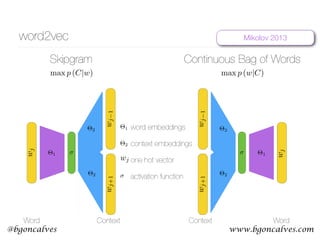
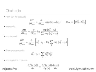
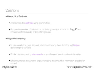
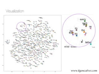
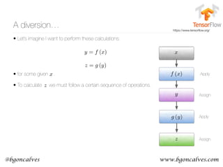
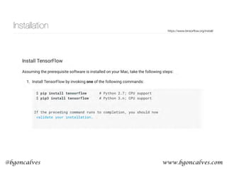
Cross-Entropy
• First we have to recall that what we are, in effect, comparing two probability distributions:
• and the one-hot encoding of the context:
• The Cross Entropy measures the distance, in number of bits, between two probability
distributions p and q:
• In our case, this becomes:
• So it’s clear that the only non zero term is the one that corresponds to the “hot” element of
• This is our Error function. But how can we use this to update the values of and ?
p (wk|wj)
H (p, q) =
X
k
pk log qk
H = log p (wj+1|wj)
wj+1
wj+1 = (0, 0, 0, 1, 0, 0, · · · )
T
H [wj+1, p (wk|wj)] =
X
k
wk
j+1 log p (wk|wj)
⇥1 ⇥2](https://image.slidesharecdn.com/word2vecoreillyai-171121190816/85/Word2vec-and-Friends-8-320.jpg)


![www.bgoncalves.com@bgoncalves
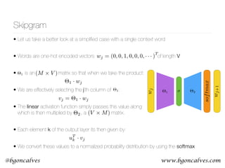
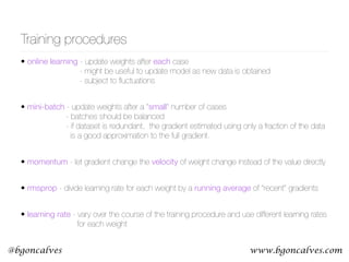
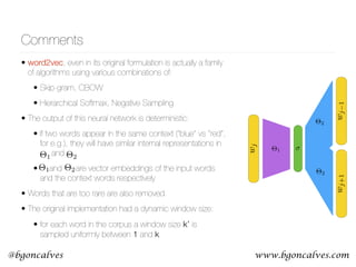
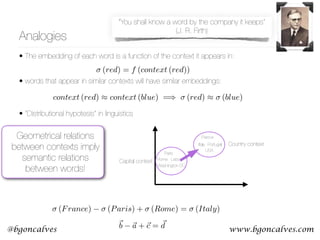
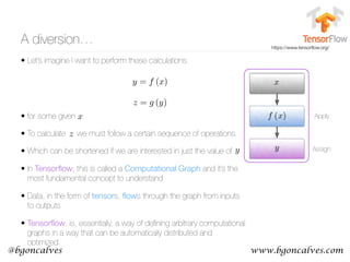
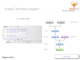
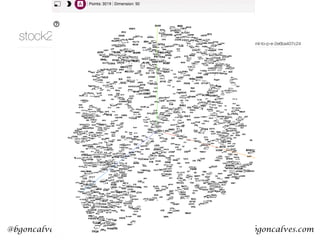
Linguistic Change
• Train word embeddings for different years using
Google Books
• Independently trained embeddings differ by an
arbitrary rotation
• Align the different embeddings for different years
• Track the way in which the meaning of words shifted
over time!
Statistically Significant Detection of Linguistic Change
Vivek Kulkarni
Stony Brook University, USA
vvkulkarni@cs.stonybrook.edu
Rami Al-Rfou
Stony Brook University, USA
ralrfou@cs.stonybrook.edu
Bryan Perozzi
Stony Brook University, USA
bperozzi@cs.stonybrook.edu
Steven Skiena
Stony Brook University, USA
skiena@cs.stonybrook.edu
ABSTRACT
We propose a new computational approach for tracking and
detecting statistically significant linguistic shifts in the mean-
ing and usage of words. Such linguistic shifts are especially
prevalent on the Internet, where the rapid exchange of ideas
can quickly change a word’s meaning. Our meta-analysis
approach constructs property time series of word usage, and
then uses statistically sound change point detection algo-
rithms to identify significant linguistic shifts.
We consider and analyze three approaches of increasing
complexity to generate such linguistic property time series,
the culmination of which uses distributional characteristics
inferred from word co-occurrences. Using recently proposed
deep neural language models, we first train vector represen-
tations of words for each time period. Second, we warp the
vector spaces into one unified coordinate system. Finally, we
construct a distance-based distributional time series for each
word to track its linguistic displacement over time.
We demonstrate that our approach is scalable by track-
ing linguistic change across years of micro-blogging using
Twitter, a decade of product reviews using a corpus of movie
reviews from Amazon, and a century of written books using
the Google Book Ngrams. Our analysis reveals interesting
patterns of language usage change commensurate with each
medium.
Categories and Subject Descriptors
H.3.3 [Information Storage and Retrieval]: Information
Search and Retrieval
Keywords
Web Mining;Computational Linguistics
1. INTRODUCTION
Natural languages are inherently dynamic, evolving over
time to accommodate the needs of their speakers. This
e↵ect is especially prevalent on the Internet, where the rapid
exchange of ideas can change a word’s meaning overnight.
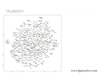
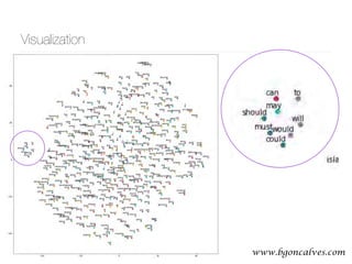
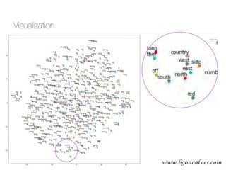
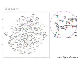
Figure 1: A 2-dimensional projection of the latent seman-
tic space captured by our algorithm. Notice the semantic
trajectory of the word gay transitioning meaning in the space.
In this paper, we study the problem of detecting such
linguistic shifts on a variety of media including micro-blog
posts, product reviews, and books. Specifically, we seek to
detect the broadening and narrowing of semantic senses of
words, as they continually change throughout the lifetime of
a medium.
We propose the first computational approach for track-
ing and detecting statistically significant linguistic shifts of
words. To model the temporal evolution of natural language,
we construct a time series per word. We investigate three
methods to build our word time series. First, we extract
Frequency based statistics to capture sudden changes in word
usage. Second, we construct Syntactic time series by ana-
lyzing each word’s part of speech (POS) tag distribution.
Finally, we infer contextual cues from word co-occurrence
statistics to construct Distributional time series. In order to
detect and establish statistical significance of word changes
over time, we present a change point detection algorithm,
which is compatible with all methods.
Figure 1 illustrates a 2-dimensional projection of the latent
semantic space captured by our Distributional method. We
clearly observe the sequence of semantic shifts that the word
gay has undergone over the last century (1900-2005). Ini-
tially, gay was an adjective that meant cheerful or dapper.
WWW’15, 625 (2015)Statistically Significant Detection of Linguistic Change
Vivek Kulkarni
Stony Brook University, USA
vvkulkarni@cs.stonybrook.edu
Rami Al-Rfou
Stony Brook University, USA
ralrfou@cs.stonybrook.edu
Bryan Perozzi
Stony Brook University, USA
bperozzi@cs.stonybrook.edu
Steven Skiena
Stony Brook University, USA
skiena@cs.stonybrook.edu
ABSTRACT
We propose a new computational approach for tracking and
detecting statistically significant linguistic shifts in the mean-
ing and usage of words. Such linguistic shifts are especially
prevalent on the Internet, where the rapid exchange of ideas
can quickly change a word’s meaning. Our meta-analysis
approach constructs property time series of word usage, and
then uses statistically sound change point detection algo-
rithms to identify significant linguistic shifts.
We consider and analyze three approaches of increasing
complexity to generate such linguistic property time series,
the culmination of which uses distributional characteristics
inferred from word co-occurrences. Using recently proposed
deep neural language models, we first train vector represen-
tations of words for each time period. Second, we warp the
vector spaces into one unified coordinate system. Finally, we
construct a distance-based distributional time series for each
word to track its linguistic displacement over time.
We demonstrate that our approach is scalable by track-
ing linguistic change across years of micro-blogging using
Twitter, a decade of product reviews using a corpus of movie
reviews from Amazon, and a century of written books using
talkative
profligate
courageous
apparitional
dapper
sublimely
unembarrassed
courteous
sorcerers
metonymy
religious
adolescents
philanthropist
illiterate
transgendered
artisans
healthy
gays
homosexual
transgender
lesbian
statesman
hispanic
uneducated
gay1900
gay1950
gay1975
gay1990
gay2005
cheerful
Figure 1: A 2-dimensional projection of the latent seman-
tic space captured by our algorithm. Notice the semantic
trajectory of the word gay transitioning meaning in the space.
In this paper, we study the problem of detecting such
linguistic shifts on a variety of media including micro-blog
posts, product reviews, and books. Specifically, we seek to](https://image.slidesharecdn.com/word2vecoreillyai-171121190816/85/Word2vec-and-Friends-35-320.jpg)
![www.bgoncalves.com@bgoncalves
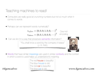
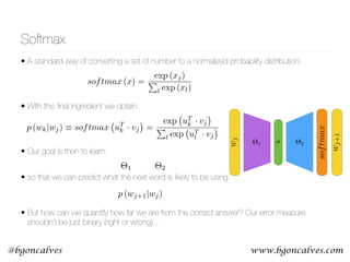
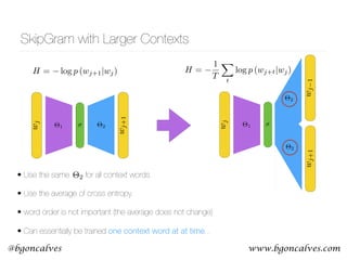
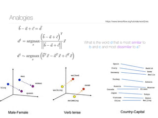
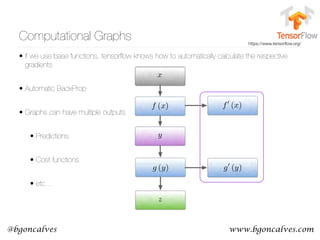
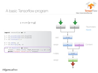
node2vec
• You can generate a graph out of a sequence of words by assigning a node to each word and
connecting the words within their neighbors through edges.
• With this representation, a piece of text is a walk through the network. Then perhaps we can
invert the process? Use walks through a network to generate a sequence of nodes that can
be used to train node embeddings?
• node embeddings should capture features of the network structure and allow for detection of
similarities between nodes.
node2vec: Scalable Feature Learning for Networks
Aditya Grover
Stanford University
adityag@cs.stanford.edu
Jure Leskovec
Stanford University
jure@cs.stanford.edu
ABSTRACT
Prediction tasks over nodes and edges in networks require careful
effort in engineering features used by learning algorithms. Recent
research in the broader field of representation learning has led to
significant progress in automating prediction by learning the fea-
tures themselves. However, present feature learning approaches
are not expressive enough to capture the diversity of connectivity
patterns observed in networks.
Here we propose node2vec, an algorithmic framework for learn-
ing continuous feature representations for nodes in networks. In
node2vec, we learn a mapping of nodes to a low-dimensional space
of features that maximizes the likelihood of preserving network
neighborhoods of nodes. We define a flexible notion of a node’s
network neighborhood and design a biased random walk procedure,
which efficiently explores diverse neighborhoods. Our algorithm
generalizes prior work which is based on rigid notions of network
neighborhoods, and we argue that the added flexibility in exploring
neighborhoods is the key to learning richer representations.
We demonstrate the efficacy of node2vec over existing state-of-
the-art techniques on multi-label classification and link prediction
in several real-world networks from diverse domains. Taken to-
gether, our work represents a new way for efficiently learning state-
of-the-art task-independent representations in complex networks.
Categories and Subject Descriptors: H.2.8 [Database Manage-
ment]: Database applications—Data mining; I.2.6 [Artificial In-
telligence]: Learning
General Terms: Algorithms; Experimentation.
Keywords: Information networks, Feature learning, Node embed-
dings, Graph representations.
1. INTRODUCTION
Many important tasks in network analysis involve predictions
over nodes and edges. In a typical node classification task, we
are interested in predicting the most probable labels of nodes in
a network [33]. For example, in a social network, we might be
interested in predicting interests of users, or in a protein-protein in-
teraction network we might be interested in predicting functional
labels of proteins [25, 37]. Similarly, in link prediction, we wish to
Permission to make digital or hard copies of all or part of this work for personal or
classroom use is granted without fee provided that copies are not made or distributed
predict whether a pair of nodes in a network should have an edge
connecting them [18]. Link prediction is useful in a wide variety
of domains; for instance, in genomics, it helps us discover novel
interactions between genes, and in social networks, it can identify
real-world friends [2, 34].
Any supervised machine learning algorithm requires a set of in-
formative, discriminating, and independent features. In prediction
problems on networks this means that one has to construct a feature
vector representation for the nodes and edges. A typical solution in-
volves hand-engineering domain-specific features based on expert
knowledge. Even if one discounts the tedious effort required for
feature engineering, such features are usually designed for specific
tasks and do not generalize across different prediction tasks.
An alternative approach is to learn feature representations by
solving an optimization problem [4]. The challenge in feature learn-
ing is defining an objective function, which involves a trade-off
in balancing computational efficiency and predictive accuracy. On
one side of the spectrum, one could directly aim to find a feature
representation that optimizes performance of a downstream predic-
tion task. While this supervised procedure results in good accu-
racy, it comes at the cost of high training time complexity due to a
blowup in the number of parameters that need to be estimated. At
the other extreme, the objective function can be defined to be inde-
pendent of the downstream prediction task and the representations
can be learned in a purely unsupervised way. This makes the op-
timization computationally efficient and with a carefully designed
objective, it results in task-independent features that closely match
task-specific approaches in predictive accuracy [21, 23].
However, current techniques fail to satisfactorily define and opti-
mize a reasonable objective required for scalable unsupervised fea-
ture learning in networks. Classic approaches based on linear and
non-linear dimensionality reduction techniques such as Principal
Component Analysis, Multi-Dimensional Scaling and their exten-
sions [3, 27, 30, 35] optimize an objective that transforms a repre-
sentative data matrix of the network such that it maximizes the vari-
ance of the data representation. Consequently, these approaches in-
variably involve eigendecomposition of the appropriate data matrix
which is expensive for large real-world networks. Moreover, the
resulting latent representations give poor performance on various
prediction tasks over networks.
Alternatively, we can design an objective that seeks to preserve
local neighborhoods of nodes. The objective can be efficiently op-
arXiv:1607.00653v1[cs.SI]3Jul2016
KDD’16, 855 (2016)](https://image.slidesharecdn.com/word2vecoreillyai-171121190816/85/Word2vec-and-Friends-36-320.jpg)
![www.bgoncalves.com@bgoncalves
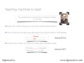
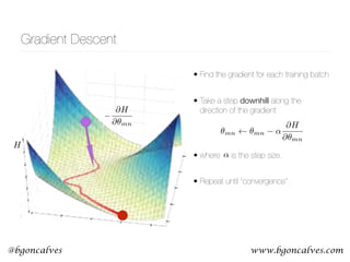
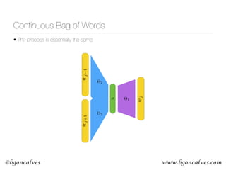
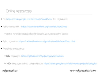
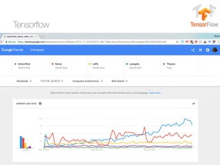
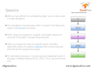
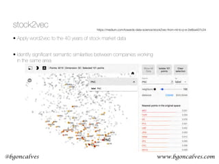
node2vec
• The features depends strongly on the way in which the network is
traversed
• Generate the contexts for each node using Breath First Search and
Depth First Search
• Perform a biased Random Walk
KDD’16, 855 (2016)
n communities they belong to (i.e., ho-
he organization could be based on the
n the network (i.e., structural equiva-
tance, in Figure 1, we observe nodes
ame tightly knit community of nodes,
the two distinct communities share the
node. Real-world networks commonly
uivalences. Thus, it is essential to allow
can learn node representations obeying
earn representations that embed nodes
mmunity closely together, as well as to
nodes that share similar roles have sim-
d allow feature learning algorithms to
iety of domains and prediction tasks.
node2vec, a semi-supervised algorithm
g in networks. We optimize a custom
on using SGD motivated by prior work
ing [21]. Intuitively, our approach re-
s that maximize the likelihood of pre-
oods of nodes in a d-dimensional fea-
der random walk approach to generate
hoods for nodes.
n defining a flexible notion of a node’s
y choosing an appropriate notion of a
an learn representations that organize
ork roles and/or communities they be-
u
s3
s2
s1
s4
s8
s9
s6
s7
s5
BFS
DFS
Figure 1: BFS and DFS search strategies from node u (k = 3).
principles in network science, providing flexibility in discov-
ering representations conforming to different equivalences.
3. We extend node2vec and other feature learning methods based
on neighborhood preserving objectives, from nodes to pairs
of nodes for edge-based prediction tasks.
4. We empirically evaluate node2vec for multi-label classifica-
tion and link prediction on several real-world datasets.
The rest of the paper is structured as follows. In Section 2, we
briefly survey related work in feature learning for networks. We
present the technical details for feature learning using node2vec
in Section 3. In Section 4, we empirically evaluate node2vec on
prediction tasks over nodes and edges on various real-world net-
works and assess the parameter sensitivity, perturbation analysis,
and scalability aspects of our algorithm. We conclude with a dis-
cussion of the node2vec framework and highlight some promis-
ing directions for future work in Section 5. Datasets and a refer-
ain structural equivalence, it is of-
e local neighborhoods accurately.
nce based on network roles such as
d just by observing the immediate
restricting search to nearby nodes,
on and obtains a microscopic view
ode. Additionally, in BFS, nodes in
d to repeat many times. This is also
ance in characterizing the distribu-
t the source node. However, a very
plored for any given k.
which can explore larger parts of
t
x2
x1
v
x3
α=1
α=1/q
α=1/q
α=1/p
v
α=1
α=1/q
α=1/q
α=1/p
x2
x3t
x1
Figure 2: Illustration of the random walk procedure in node2vec.
The walk just transitioned from t to v and is now evaluating its next
• BFS - Explores only
limited neighborhoods.
Suitable for structural
equivalences
• DFS - Freely explores
neighborhoods and
covers homophiles
communities
• By modifying the
parameter of the model it
can interpolate between
the BFS and DFS
extremes](https://image.slidesharecdn.com/word2vecoreillyai-171121190816/85/Word2vec-and-Friends-37-320.jpg)
![www.bgoncalves.com@bgoncalves
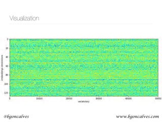
dna2vec
• Separate the genome into long non-overlapping DNS fragments.
• Convert long DNA fragments into overlapping variable length k-mers
• Train embeddings of each k-mer using Gensim implementation of SkipGram.
• Summing embeddings is related to concatenating k-mers
• Cosign similarity of k-mer embeddings reproduces a biologically motivated
similarity score (Needleman-Wunsch) that is used to align nucleoti
dna2vec: Consistent vector representations of
variable-length k-mers
Patrick Ng
ppn3@cs.cornell.edu
Abstract
One of the ubiquitous representation of long DNA sequence is dividing it into shorter k-mer components.
Unfortunately, the straightforward vector encoding of k-mer as a one-hot vector is vulnerable to the
curse of dimensionality. Worse yet, the distance between any pair of one-hot vectors is equidistant. This
is particularly problematic when applying the latest machine learning algorithms to solve problems in
biological sequence analysis. In this paper, we propose a novel method to train distributed representations
of variable-length k-mers. Our method is based on the popular word embedding model word2vec, which
is trained on a shallow two-layer neural network. Our experiments provide evidence that the summing
of dna2vec vectors is akin to nucleotides concatenation. We also demonstrate that there is correlation
between Needleman-Wunsch similarity score and cosine similarity of dna2vec vectors.
1 Introduction
The usage of k-mer representation has been a popular approach in analyzing long sequence of DNA fragments.
The k-mer representation is simple to understand and compute. Unfortunately, its straightforward vector
encoding as a one-hot vector (i.e. bit vector that consists of all zeros except for a single dimension) is
vulnerable to curse of dimensionality. Specifically, its one-hot vector has dimension exponential to the length
of k. For example, an 8-mer needs a bit vector of dimension 48
= 65536. This is problematic when applying
the latest machine learning algorithms to solve problems in biological sequence analysis, due to the fact that
most of these tools prefer lower-dimensional continuous vectors as input (Suykens and Vandewalle, 1999;
Angermueller et al., 2016; Turian et al., 2010). Worse yet, the distance between any arbitrary pair of one-hot
vectors is equidistant, even though ATGGC should be closer to ATGGG than CACGA.
1.1 Word embeddings
The Natural Language Processing (NLP) research community has a long tradition of using bag-of-words with
one-hot vector, where its dimension is equal to the vocabulary size. Recently, there has been an explosion of
using word embeddings as inputs to machine learning algorithms, especially in the deep learning community
(Mikolov et al., 2013b; LeCun et al., 2015; Bengio et al., 2013). Word embeddings are vectors of real numbers
that are distributed representations of words.
A popular training technique for word embeddings, word2vec (Mikolov et al., 2013a), consists of using a
2-layer neural network that is trained on the current word and its surrounding context words (see Section
2.3). This reconstruction of context of words is loosely inspired by the linguistic concept of distributional
hypothesis, which states that words that appear in the same context have similar meaning (Harris, 1954).
Deep learning algorithms applied with word embeddings have had dramatic improvements in the areas of
machine translation (Sutskever et al., 2014; Bahdanau et al., 2014; Cho et al., 2014), summarization (Chopra
arXiv:1701.06279v1[q-bio.QM]23Jan2017
arXiv: 1701.06279 (2017)](https://image.slidesharecdn.com/word2vecoreillyai-171121190816/85/Word2vec-and-Friends-38-320.jpg)


The document discusses methods for representing words numerically through techniques like word2vec, which allows machines to understand the context and semantics of words. It explains processes such as one-hot encoding, skip-gram, and continuous bag of words for training word embeddings, as well as algorithms for updating weights and detecting linguistic shifts over time. The research also highlights applications of tracking changes in word meanings using various mediums, demonstrating the dynamic nature of language, particularly on the internet.


![[Yang, Downey and Boyd-Graber 2015] Efficient Methods for Incorporating Knowl...](https://cdn.slidesharecdn.com/ss_thumbnails/sparse-constrained-lda-151024072334-lva1-app6891-thumbnail.jpg?width=640&height=640&fit=bounds)