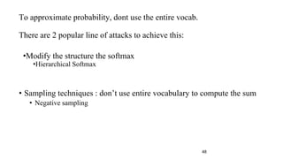
Downloaded 118 times
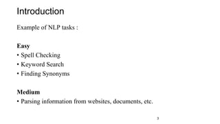

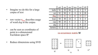
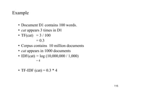
![• Given a matrix of m × n dimensionality, construct a m × k matrix, where k << n
• M = U Σ VT
• U is an m × m orthogonal matrix (UUT = I)
• Σ is a m × n diagonal matrix, with diagonal values ordered from largest to smallest (σ1 ≥
σ2 ≥ · · · ≥ σr ≥ 0, where r = min(m, n)) [σi’s are known as singular values]
• V is an n × n orthogonal matrix (VVT = I)
• We construct M’ s.t. rank(M’) = k
• We compute M’ = U Σ’ V, where Σ’ = Σ with k largest singular values
• k captures desired percentage variance
• Then, submatrix U v,k is our desired word embedding matrix.
14](https://image.slidesharecdn.com/dlblrtalk-170528144612/85/DLBLR-talk-14-320.jpg)

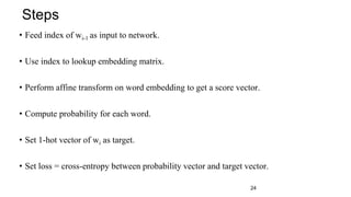


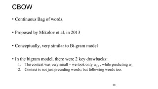
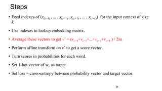
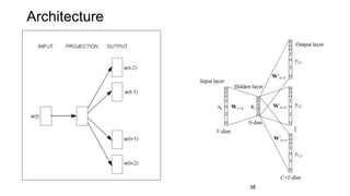


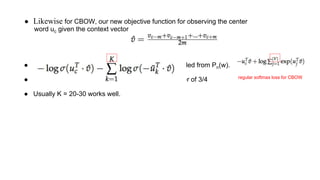

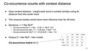
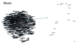
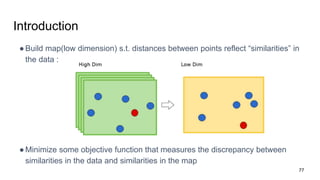
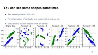


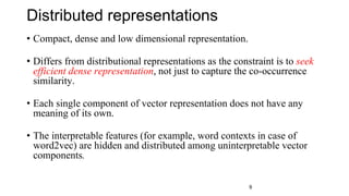
This document provides an overview and introduction to representation learning of text, specifically word vectors. It discusses older techniques like bag-of-words and n-grams, and then introduces modern distributed representations like word2vec's CBOW and Skip-Gram models as well as the GloVe model. The document covers how these models work, are evaluated, and techniques to speed them up like hierarchical softmax and negative sampling.


![[KDD 2018 tutorial] End to-end goal-oriented question answering systems](https://cdn.slidesharecdn.com/ss_thumbnails/kdd2018tutorialend-to-endgoal-orientedquestionansweringsystems-180821081440-thumbnail.jpg?width=640&height=640&fit=bounds)