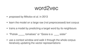
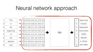
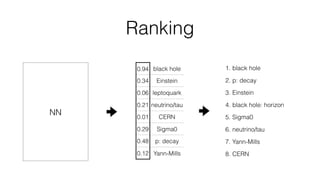
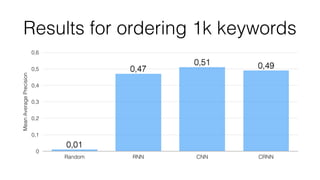
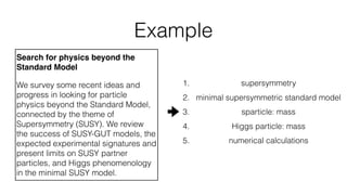
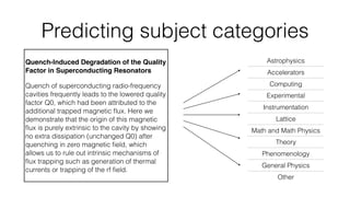
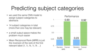
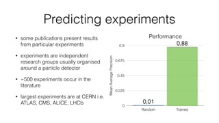
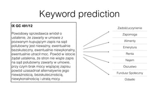
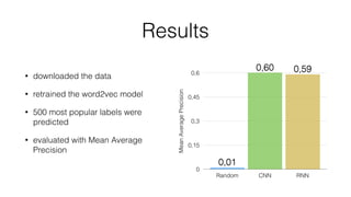
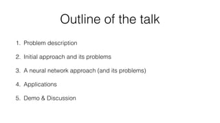
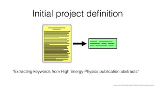
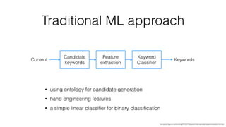
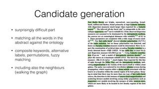
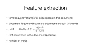
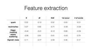
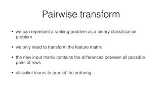
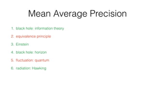
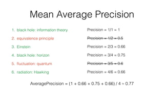
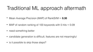
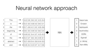
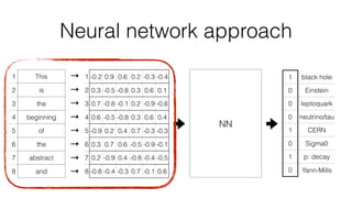
Jan Stypka
Outline of the talk
1. Problem description
2. Initial approach and its problems
3. A neural network approach (and its problems)
4. Applications
5. Demo & Discussion
Initial project definition
“Extracting keywords from High Energy Physics publication abstracts”
img source: http://bdewilde.github.io/blog/2014/09/23/intro-to-automatic-keyphrase-extraction/
Problems with keyword extraction
• What is a keyword?
• When is a keyword relevant to a text?
• What is the ground truth?
Ontology
• all possible terms in HEP
• connected with relations
• ~60k terms altogether
• ~30k used more than once
• ~10k used in practice
img source: LinkedIn network visualisations
Large training corpus
• ~200k abstracts with manually
assigned keywords since 2000
• ~300k if you include the 1990s and
papers with automatically assigned
keywords
img source:http://www.susansolovic.com/2015/05/the-paper-blizzard-despite-ecommunications/
Approaches to keyword extraction
• statistical
• linguistic
• unsupervised machine learning
• supervised machine learning
Traditional ML approach
• using ontology for candidate generation
• hand engineering features
• a simple linear classifier for binary classification
img source: blog.urx.com/urx-blog/2015/10/13/keyword-finder-automatic-keyword-extraction-from-text
Candidate generation
• surprisingly difficult part
• matching all the words in the
abstract against the ontology
• composite keywords, alternative
labels, permutations, fuzzy
matching
• including also the neighbours
(walking the graph)
Feature extraction
• term frequency (number of occurrences in this document)
• document frequency (how many documents contain this word)
• tf-idf
• first occurrence in the document (position)
• number of words
Feature extraction
tf df tfidf 1st occur # of words
quark 0.22 -0.12 0.32 0.03 -0.21
neutrino/tau 0.57 0.60 -0.71 -0.30 -0.59
Higgs:
coupling
-0.44 -0.41 -0.12 0.89 -0.28
elastic
scattering
-0.90 0.91 0.43 -0.43 0.79
Sigma0: mass 0.11 -0.77 -0.94 0.46 0.17
Keyword classification
tf tfidf
quark 0.22 0.32
neutrino/tau 0.57 -0.71
Higgs:
coupling
-0.44 -0.12
elastic
scattering
-0.90 0.43
Sigma0:
mass
0.11 -0.94
tf
-1
-0,5
0
0,5
1
tfidf
-1 -0,5 0 0,5 1
Keyword classification
tf tfidf
quark 0.22 0.32
neutrino/tau 0.57 -0.71
Higgs:
coupling
-0.44 -0.12
elastic
scattering
-0.90 0.43
Sigma0:
mass
0.11 -0.94
tf
-1
-0,5
0
0,5
1
tfidf
-1 -0,5 0 0,5 1
Keyword classification
tf tfidf
quark 0.22 0.32
neutrino/tau 0.57 -0.71
Higgs:
coupling
-0.44 -0.12
elastic
scattering
-0.90 0.43
Sigma0:
mass
0.11 -0.94
tf
-1
-0,5
0
0,5
1
tfidf
-1 -0,5 0 0,5 1
Ranking approach
• keywords should not be classified in isolation
• keyword relevance is not binary
• keyword extraction is a ranking problem!
• model should produce a ranking of the vocabulary for every abstract
• model learns to order all the terms by relevance to the input text
Pairwise transform
• we can represent a ranking problem as a binary classification
problem
• we only need to transform the feature matrix
• the new input matrix contains the differences between all possible
pairs of rows
• classifier learns to predict the ordering
Pairwise transform
a b c result
w1 a1 b1 c1 ✓
w2 a2 b2 c2 ✗
w3 a3 b3 c3 ✓
w4 a4 b4 c4 ✗
a b c result
w1 - w2 a1 - a2 b1 - b2 c1 - c2 ↑
w1 - w3 a1 - a3 b1 - b3 c1 - c3 ↓
w1 - w4 a1 - a4 b1 - b4 c1 - c4 ↑
w2 - w3 a2 - a3 b2 - b3 c2 - c3 ↓
w2 - w4 a2 - a4 b2 - b4 c2 - c4 ↓
w3 - w4 a3 - a4 b3 - b4 c3 - c4 ↑
Ranking result
a b c result
w1 - w2 a1 - a2 b1 - b2 c1 - c2 ↑
w1 - w3 a1 - a3 b1 - b3 c1 - c3 ↓
w1 - w4 a1 - a4 b1 - b4 c1 - c4 ↑
w2 - w3 a2 - a3 b2 - b3 c2 - c3 ↓
w2 - w4 a2 - a4 b2 - b4 c2 - c4 ↓
w3 - w4 a3 - a4 b3 - b4 c3 - c4 ↑
1. black hole: information theory
2. equivalence principle
3. Einstein
4. black hole: horizon
5. fluctuation: quantum
6. radiation: Hawking
7. density matrix
Mean Average Precision
• metric to evaluate rankings
• gives a single number
• can be used to compare different rankings of the same vocabulary
• average precision values at ranks of relevant keywords
• mean of those averages across different queries
Mean Average Precision
1. black hole: information theory
2. equivalence principle
3. Einstein
4. black hole: horizon
5. fluctuation: quantum
6. radiation: Hawking
Mean Average Precision
1. black hole: information theory
2. equivalence principle
3. Einstein
4. black hole: horizon
5. fluctuation: quantum
6. radiation: Hawking
Precision = 1/1 = 1
Precision = 1/2 = 0.5
Precision = 2/3 = 0.66
Precision = 3/4 = 0.75
Precision = 3/5 = 0.6
Precision = 4/6 = 0.66
AveragePrecision = (1 + 0.66 + 0.75 + 0.66) / 4 ≈ 0.77
Traditional ML approach aftermath
• Mean Average Precision (MAP) of RankSVM ≈ 0.30
• MAP of random ranking of 100 keywords with 5 hits ≈ 0.09
• need something better
• candidate generation is difficult, features are not meaningful
• is it possible to skip those steps?
Neural network approach
1 This
2 is
3 the
4 beginning
5 of
6 the
7 abstract
8 and
1 -0.2 0.9 0.6 0.2 -0.3 -0.4
2 0.3 -0.5 -0.8 0.3 0.6 0.1
3 0.7 -0.8 -0.1 0.2 -0.9 -0.6
4 0.6 -0.5 -0.8 0.3 0.6 0.4
5 -0.9 0.2 0.4 0.7 -0.3 -0.3
6 0.3 0.7 0.6 -0.5 -0.9 -0.1
7 0.2 -0.9 0.4 -0.8 -0.4 -0.5
8 -0.8 -0.4 -0.3 0.7 -0.1 0.6
NN
1 black hole
0 Einstein
0 leptoquark
0 neutrino/tau
1 CERN
0 Sigma0
1 p: decay
0 Yann-Mills
→
→
→
→
→
→
→
→
Word vectors
• strings for computers are meaningless tokens
• “cat” is as similar to “dog” as it is to “skyscraper”
• in vector space terms, words are vectors with one 1 and a lot of 0
• it’s major problem is:
img source: http://cs224d.stanford.edu/syllabus.html
Word vectors
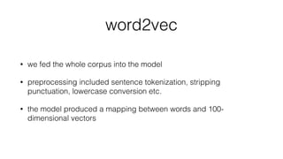
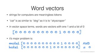
• we need to represent the meaning of the words
• we want to perform arithmetics e.g. vec[“hotel”] - vec[“motel”] ≈ 0
• we want them to be low-dimensional
• we want them to preserve relations 

e.g. vec[“Paris”] - vec[“France”] ≈ vec[“Berlin”] - vec[“Germany”]
• vec[“king”] - vec[“man”] + vec[“woman”] ≈ vec[“queen”]
word2vec
• proposed by Mikolov et al. in 2013
• learn the model on a large raw (not preprocessed) text corpus
• trains a model by predicting a target word by its neighbours
• “Piotrek _____ tomatoes” or “Gosia is a ____ sister”
• use a context window and walk it through the whole corpus
iteratively updating the vector representations
word2vec
• cost function:
• where the probabilities:
img source: http://cs224d.stanford.edu/syllabus.html
word2vec
img source: http://d.hatena.ne.jp/nishiohirokazu/20140606/1401983909
word2vec
img source: http://deeplearning4j.org/word2vec
word2vec
• we fed the whole corpus into the model
• preprocessing included sentence tokenization, stripping
punctuation, lowercase conversion etc.
• the model produced a mapping between words and 100-
dimensional vectors
Demo
Neural network approach
1 This
2 is
3 the
4 beginning
5 of
6 the
7 abstract
8 and
1 -0.2 0.9 0.6 0.2 -0.3 -0.4
2 0.3 -0.5 -0.8 0.3 0.6 0.1
3 0.7 -0.8 -0.1 0.2 -0.9 -0.6
4 0.6 -0.5 -0.8 0.3 0.6 0.4
5 -0.9 0.2 0.4 0.7 -0.3 -0.3
6 0.3 0.7 0.6 -0.5 -0.9 -0.1
7 0.2 -0.9 0.4 -0.8 -0.4 -0.5
8 -0.8 -0.4 -0.3 0.7 -0.1 0.6
NN
1 black hole
0 Einstein
0 leptoquark
0 neutrino/tau
1 CERN
0 Sigma0
1 p: decay
0 Yann-Mills
→
→
→
→
→
→
→
→
Classic Neural Networks
• just a directed graph with weighted edges
• supposed to simulate our brain architecture
• nodes are called neurons and divided into layers
• usually at least three layers - input, hidden (one or more) and output
• feed the input into the input layer, propagate the values along the
edges until the output layer
Forward propagation in NN
img source: http://picoledelimao.github.io/blog/2016/01/31/is-it-a-cat-or-dog-a-neural-network-application-in-opencv/
Neural Networks
• just adjust parameters to minimise the errors and conform to the
training data
• in theory able to approximate any function
• take a long time to train
• come in different variations e.g. recurrent neural networks and
convolutional neural networks
Recurrent Neural Networks
• classic NN have no state/memory
• RNNs try to go about this by adding
an additional matrix in every node
• computing the state of a neuron
depends on the previous layer and
on the current state (inner matrix)
• used for learning sequences
• come in different kinds e.g. LSTM or
GRU
=
img source: http://colah.github.io/
Convolutional Neural Networks
• inspired by convolutions in image
and audio processing
• you learn a set of neurons once and
reuse them to compute values from
the whole input data
• similar to convolutional filters
• very successful in image and audio
classification
img source: http://colah.github.io/
Training
• test CNN, RNN and CRNN (combination of both)
• split the data into training, test and validation set (ratio 50:25:25)
• networks try to predict 0 or 1 on every label
• use the confidence values to produce a ranking
• evaluate the ranking with Mean Average Precision
Ranking
NN
0.94 black hole
0.34 Einstein
0.06 leptoquark
0.21 neutrino/tau
0.01 CERN
0.29 Sigma0
0.48 p: decay
0.12 Yann-Mills
1. black hole
2. p: decay
3. Einstein
4. black hole: horizon
5. Sigma0
6. neutrino/tau
7. Yann-Mills
8. CERN
Results for ordering 1k keywordsMeanAveragePrecision
0
0,1
0,2
0,3
0,4
0,5
0,6
Random RNN CNN CRNN
0,490,51
0,47
0,01
Example
Search for physics beyond the
Standard Model
We survey some recent ideas and
progress in looking for particle
physics beyond the Standard Model,
connected by the theme of
Supersymmetry (SUSY). We review
the success of SUSY-GUT models, the
expected experimental signatures and
present limits on SUSY partner
particles, and Higgs phenomenology
in the minimal SUSY model.
1. supersymmetry
2. minimal supersymmetric standard model
3. sparticle: mass
4. Higgs particle: mass
5. numerical calculations
Generalisation
• keyword extraction is just a special case
• what we were actually doing was multi-label text classification i.e.
learning to assign many arbitrary labels to text
• the models can be used to do any text classification - the only
requirement is a predefined vocabulary and a large training set
Predicting subject categories
Quench-Induced Degradation of the Quality
Factor in Superconducting Resonators
Quench of superconducting radio-frequency
cavities frequently leads to the lowered quality
factor Q0, which had been attributed to the
additional trapped magnetic flux. Here we
demonstrate that the origin of this magnetic
flux is purely extrinsic to the cavity by showing
no extra dissipation (unchanged Q0) after
quenching in zero magnetic field, which
allows us to rule out intrinsic mechanisms of
flux trapping such as generation of thermal
currents or trapping of the rf field.
Astrophysics
Accelerators
Computing
Experimental
Instrumentation
Lattice
Math and Math Physics
Theory
Phenomenology
General Physics
Other
Predicting subject categories
• we used the same CNN model to
assign subject categories to
abstracts
• 14 subject categories in total 

(more than one may be relevant)
• a small output space makes the
problem much easier
• Mean Reciprocal Rank (MRR) is just
the inversion of the rank of the first
relevant label (1, ½, ⅓, ¼, ⅕ …)
Performance
0
0,25
0,5
0,75
1
MRR MAP
Random Trained Random Trained
0,920,93
0,230,23
Predicting experiments
• some publications present results
from particular experiments
• experiments are independent
research groups usually organised
around a particle detector
• ~500 experiments occur in the
literature
• largest experiments are at CERN i.e.
ATLAS, CMS, ALICE, LHCb
Performance
MeanAveragePrecision
0
0,225
0,45
0,675
0,9
Random Trained
0,88
0,01
Court rulings
Keyword prediction for Polish civil court rulings
Keyword prediction
IX GC 491/12
Powodowy sprzedawca wniósł o
ustalenie, że zawarty w umowie z
pozwanym kupującym zapis na sąd
polubowny jest nieważny, ewentualnie
bezskuteczny, ewentualnie niewykonalny,
ewentualnie utracił moc. Powód w istocie
żądał ustalenia, że stron nie wiąże zapis
na sąd polubowny zawarty w umowie,
przy czym brak mocy wiążącej zapisu
powód uzasadniał alternatywnie jego
nieważnością, bezskutecznością,
niewykonalnością i utratą mocy.
Zadośćuczynienie
Zapomoga
Alimenty
Emerytura
Renta
Najem
Oszustwo
Fundusz Społeczny
Odsetki
Results
• downloaded the data
• retrained the word2vec model
• 500 most popular labels were
predicted
• evaluated with Mean Average
Precision
MeanAveragePrecision
0
0,15
0,3
0,45
0,6
Random CNN RNN
0,590,60
0,01
Demo
Technologies
• word2vec models have been trained using the gensim library
• keras framework was used to build neural network models
• keras uses Theano or TensorFlow for the heavy-lifting calculations
• python
Acknowledgements
• dr Eamonn Maguire
• dr Gilles Louppe
• RCS-SIS-OA group @ CERN
Resources
• magpie.inspirehep.net
• github.com/inspirehep/magpie
• github.com/inspirehep/inspire-magpie
• bdewilde.github.io/blog/2014/09/23/intro-to-automatic-keyphrase-extraction
• cs224d.stanford.edu
• colah.github.io
• fa.bianp.net/blog/2012/learning-to-rank-with-scikit-learn-the-pairwise-transform
Thanks!
@ janstypka at gmail.com
github.com/jstypka
linkedin.com/in/jstypka

Magpie

  • 1.
  • 2.
    Outline of thetalk 1. Problem description 2. Initial approach and its problems 3. A neural network approach (and its problems) 4. Applications 5. Demo & Discussion
  • 3.
    Initial project definition “Extractingkeywords from High Energy Physics publication abstracts” img source: http://bdewilde.github.io/blog/2014/09/23/intro-to-automatic-keyphrase-extraction/
  • 4.
    Problems with keywordextraction • What is a keyword? • When is a keyword relevant to a text? • What is the ground truth?
  • 5.
    Ontology • all possibleterms in HEP • connected with relations • ~60k terms altogether • ~30k used more than once • ~10k used in practice img source: LinkedIn network visualisations
  • 6.
    Large training corpus •~200k abstracts with manually assigned keywords since 2000 • ~300k if you include the 1990s and papers with automatically assigned keywords img source:http://www.susansolovic.com/2015/05/the-paper-blizzard-despite-ecommunications/
  • 7.
    Approaches to keywordextraction • statistical • linguistic • unsupervised machine learning • supervised machine learning
  • 8.
    Traditional ML approach •using ontology for candidate generation • hand engineering features • a simple linear classifier for binary classification img source: blog.urx.com/urx-blog/2015/10/13/keyword-finder-automatic-keyword-extraction-from-text
  • 9.
    Candidate generation • surprisinglydifficult part • matching all the words in the abstract against the ontology • composite keywords, alternative labels, permutations, fuzzy matching • including also the neighbours (walking the graph)
  • 10.
    Feature extraction • termfrequency (number of occurrences in this document) • document frequency (how many documents contain this word) • tf-idf • first occurrence in the document (position) • number of words
  • 11.
    Feature extraction tf dftfidf 1st occur # of words quark 0.22 -0.12 0.32 0.03 -0.21 neutrino/tau 0.57 0.60 -0.71 -0.30 -0.59 Higgs: coupling -0.44 -0.41 -0.12 0.89 -0.28 elastic scattering -0.90 0.91 0.43 -0.43 0.79 Sigma0: mass 0.11 -0.77 -0.94 0.46 0.17
  • 12.
    Keyword classification tf tfidf quark0.22 0.32 neutrino/tau 0.57 -0.71 Higgs: coupling -0.44 -0.12 elastic scattering -0.90 0.43 Sigma0: mass 0.11 -0.94 tf -1 -0,5 0 0,5 1 tfidf -1 -0,5 0 0,5 1
  • 13.
    Keyword classification tf tfidf quark0.22 0.32 neutrino/tau 0.57 -0.71 Higgs: coupling -0.44 -0.12 elastic scattering -0.90 0.43 Sigma0: mass 0.11 -0.94 tf -1 -0,5 0 0,5 1 tfidf -1 -0,5 0 0,5 1
  • 14.
    Keyword classification tf tfidf quark0.22 0.32 neutrino/tau 0.57 -0.71 Higgs: coupling -0.44 -0.12 elastic scattering -0.90 0.43 Sigma0: mass 0.11 -0.94 tf -1 -0,5 0 0,5 1 tfidf -1 -0,5 0 0,5 1
  • 15.
    Ranking approach • keywordsshould not be classified in isolation • keyword relevance is not binary • keyword extraction is a ranking problem! • model should produce a ranking of the vocabulary for every abstract • model learns to order all the terms by relevance to the input text
  • 16.
    Pairwise transform • wecan represent a ranking problem as a binary classification problem • we only need to transform the feature matrix • the new input matrix contains the differences between all possible pairs of rows • classifier learns to predict the ordering
  • 17.
    Pairwise transform a bc result w1 a1 b1 c1 ✓ w2 a2 b2 c2 ✗ w3 a3 b3 c3 ✓ w4 a4 b4 c4 ✗ a b c result w1 - w2 a1 - a2 b1 - b2 c1 - c2 ↑ w1 - w3 a1 - a3 b1 - b3 c1 - c3 ↓ w1 - w4 a1 - a4 b1 - b4 c1 - c4 ↑ w2 - w3 a2 - a3 b2 - b3 c2 - c3 ↓ w2 - w4 a2 - a4 b2 - b4 c2 - c4 ↓ w3 - w4 a3 - a4 b3 - b4 c3 - c4 ↑
  • 18.
    Ranking result a bc result w1 - w2 a1 - a2 b1 - b2 c1 - c2 ↑ w1 - w3 a1 - a3 b1 - b3 c1 - c3 ↓ w1 - w4 a1 - a4 b1 - b4 c1 - c4 ↑ w2 - w3 a2 - a3 b2 - b3 c2 - c3 ↓ w2 - w4 a2 - a4 b2 - b4 c2 - c4 ↓ w3 - w4 a3 - a4 b3 - b4 c3 - c4 ↑ 1. black hole: information theory 2. equivalence principle 3. Einstein 4. black hole: horizon 5. fluctuation: quantum 6. radiation: Hawking 7. density matrix
  • 19.
    Mean Average Precision •metric to evaluate rankings • gives a single number • can be used to compare different rankings of the same vocabulary • average precision values at ranks of relevant keywords • mean of those averages across different queries
  • 20.
    Mean Average Precision 1.black hole: information theory 2. equivalence principle 3. Einstein 4. black hole: horizon 5. fluctuation: quantum 6. radiation: Hawking
  • 21.
    Mean Average Precision 1.black hole: information theory 2. equivalence principle 3. Einstein 4. black hole: horizon 5. fluctuation: quantum 6. radiation: Hawking Precision = 1/1 = 1 Precision = 1/2 = 0.5 Precision = 2/3 = 0.66 Precision = 3/4 = 0.75 Precision = 3/5 = 0.6 Precision = 4/6 = 0.66 AveragePrecision = (1 + 0.66 + 0.75 + 0.66) / 4 ≈ 0.77
  • 22.
    Traditional ML approachaftermath • Mean Average Precision (MAP) of RankSVM ≈ 0.30 • MAP of random ranking of 100 keywords with 5 hits ≈ 0.09 • need something better • candidate generation is difficult, features are not meaningful • is it possible to skip those steps?
  • 23.
    Neural network approach 1This 2 is 3 the 4 beginning 5 of 6 the 7 abstract 8 and 1 -0.2 0.9 0.6 0.2 -0.3 -0.4 2 0.3 -0.5 -0.8 0.3 0.6 0.1 3 0.7 -0.8 -0.1 0.2 -0.9 -0.6 4 0.6 -0.5 -0.8 0.3 0.6 0.4 5 -0.9 0.2 0.4 0.7 -0.3 -0.3 6 0.3 0.7 0.6 -0.5 -0.9 -0.1 7 0.2 -0.9 0.4 -0.8 -0.4 -0.5 8 -0.8 -0.4 -0.3 0.7 -0.1 0.6 NN 1 black hole 0 Einstein 0 leptoquark 0 neutrino/tau 1 CERN 0 Sigma0 1 p: decay 0 Yann-Mills → → → → → → → →
  • 24.
    Neural network approach 1This 2 is 3 the 4 beginning 5 of 6 the 7 abstract 8 and 1 -0.2 0.9 0.6 0.2 -0.3 -0.4 2 0.3 -0.5 -0.8 0.3 0.6 0.1 3 0.7 -0.8 -0.1 0.2 -0.9 -0.6 4 0.6 -0.5 -0.8 0.3 0.6 0.4 5 -0.9 0.2 0.4 0.7 -0.3 -0.3 6 0.3 0.7 0.6 -0.5 -0.9 -0.1 7 0.2 -0.9 0.4 -0.8 -0.4 -0.5 8 -0.8 -0.4 -0.3 0.7 -0.1 0.6 NN 1 black hole 0 Einstein 0 leptoquark 0 neutrino/tau 1 CERN 0 Sigma0 1 p: decay 0 Yann-Mills → → → → → → → →
  • 25.
    Word vectors • stringsfor computers are meaningless tokens • “cat” is as similar to “dog” as it is to “skyscraper” • in vector space terms, words are vectors with one 1 and a lot of 0 • it’s major problem is: img source: http://cs224d.stanford.edu/syllabus.html
  • 26.
    Word vectors • weneed to represent the meaning of the words • we want to perform arithmetics e.g. vec[“hotel”] - vec[“motel”] ≈ 0 • we want them to be low-dimensional • we want them to preserve relations 
 e.g. vec[“Paris”] - vec[“France”] ≈ vec[“Berlin”] - vec[“Germany”] • vec[“king”] - vec[“man”] + vec[“woman”] ≈ vec[“queen”]
  • 27.
    word2vec • proposed byMikolov et al. in 2013 • learn the model on a large raw (not preprocessed) text corpus • trains a model by predicting a target word by its neighbours • “Piotrek _____ tomatoes” or “Gosia is a ____ sister” • use a context window and walk it through the whole corpus iteratively updating the vector representations
  • 28.
    word2vec • cost function: •where the probabilities: img source: http://cs224d.stanford.edu/syllabus.html
  • 29.
  • 30.
  • 31.
    word2vec • we fedthe whole corpus into the model • preprocessing included sentence tokenization, stripping punctuation, lowercase conversion etc. • the model produced a mapping between words and 100- dimensional vectors
  • 32.
  • 33.
    Neural network approach 1This 2 is 3 the 4 beginning 5 of 6 the 7 abstract 8 and 1 -0.2 0.9 0.6 0.2 -0.3 -0.4 2 0.3 -0.5 -0.8 0.3 0.6 0.1 3 0.7 -0.8 -0.1 0.2 -0.9 -0.6 4 0.6 -0.5 -0.8 0.3 0.6 0.4 5 -0.9 0.2 0.4 0.7 -0.3 -0.3 6 0.3 0.7 0.6 -0.5 -0.9 -0.1 7 0.2 -0.9 0.4 -0.8 -0.4 -0.5 8 -0.8 -0.4 -0.3 0.7 -0.1 0.6 NN 1 black hole 0 Einstein 0 leptoquark 0 neutrino/tau 1 CERN 0 Sigma0 1 p: decay 0 Yann-Mills → → → → → → → →
  • 34.
    Classic Neural Networks •just a directed graph with weighted edges • supposed to simulate our brain architecture • nodes are called neurons and divided into layers • usually at least three layers - input, hidden (one or more) and output • feed the input into the input layer, propagate the values along the edges until the output layer
  • 35.
    Forward propagation inNN img source: http://picoledelimao.github.io/blog/2016/01/31/is-it-a-cat-or-dog-a-neural-network-application-in-opencv/
  • 36.
    Neural Networks • justadjust parameters to minimise the errors and conform to the training data • in theory able to approximate any function • take a long time to train • come in different variations e.g. recurrent neural networks and convolutional neural networks
  • 37.
    Recurrent Neural Networks •classic NN have no state/memory • RNNs try to go about this by adding an additional matrix in every node • computing the state of a neuron depends on the previous layer and on the current state (inner matrix) • used for learning sequences • come in different kinds e.g. LSTM or GRU = img source: http://colah.github.io/
  • 38.
    Convolutional Neural Networks •inspired by convolutions in image and audio processing • you learn a set of neurons once and reuse them to compute values from the whole input data • similar to convolutional filters • very successful in image and audio classification img source: http://colah.github.io/
  • 39.
    Training • test CNN,RNN and CRNN (combination of both) • split the data into training, test and validation set (ratio 50:25:25) • networks try to predict 0 or 1 on every label • use the confidence values to produce a ranking • evaluate the ranking with Mean Average Precision
  • 40.
    Ranking NN 0.94 black hole 0.34Einstein 0.06 leptoquark 0.21 neutrino/tau 0.01 CERN 0.29 Sigma0 0.48 p: decay 0.12 Yann-Mills 1. black hole 2. p: decay 3. Einstein 4. black hole: horizon 5. Sigma0 6. neutrino/tau 7. Yann-Mills 8. CERN
  • 41.
    Results for ordering1k keywordsMeanAveragePrecision 0 0,1 0,2 0,3 0,4 0,5 0,6 Random RNN CNN CRNN 0,490,51 0,47 0,01
  • 42.
    Example Search for physicsbeyond the Standard Model We survey some recent ideas and progress in looking for particle physics beyond the Standard Model, connected by the theme of Supersymmetry (SUSY). We review the success of SUSY-GUT models, the expected experimental signatures and present limits on SUSY partner particles, and Higgs phenomenology in the minimal SUSY model. 1. supersymmetry 2. minimal supersymmetric standard model 3. sparticle: mass 4. Higgs particle: mass 5. numerical calculations
  • 43.
    Generalisation • keyword extractionis just a special case • what we were actually doing was multi-label text classification i.e. learning to assign many arbitrary labels to text • the models can be used to do any text classification - the only requirement is a predefined vocabulary and a large training set
  • 44.
    Predicting subject categories Quench-InducedDegradation of the Quality Factor in Superconducting Resonators Quench of superconducting radio-frequency cavities frequently leads to the lowered quality factor Q0, which had been attributed to the additional trapped magnetic flux. Here we demonstrate that the origin of this magnetic flux is purely extrinsic to the cavity by showing no extra dissipation (unchanged Q0) after quenching in zero magnetic field, which allows us to rule out intrinsic mechanisms of flux trapping such as generation of thermal currents or trapping of the rf field. Astrophysics Accelerators Computing Experimental Instrumentation Lattice Math and Math Physics Theory Phenomenology General Physics Other
  • 45.
    Predicting subject categories •we used the same CNN model to assign subject categories to abstracts • 14 subject categories in total 
 (more than one may be relevant) • a small output space makes the problem much easier • Mean Reciprocal Rank (MRR) is just the inversion of the rank of the first relevant label (1, ½, ⅓, ¼, ⅕ …) Performance 0 0,25 0,5 0,75 1 MRR MAP Random Trained Random Trained 0,920,93 0,230,23
  • 46.
    Predicting experiments • somepublications present results from particular experiments • experiments are independent research groups usually organised around a particle detector • ~500 experiments occur in the literature • largest experiments are at CERN i.e. ATLAS, CMS, ALICE, LHCb Performance MeanAveragePrecision 0 0,225 0,45 0,675 0,9 Random Trained 0,88 0,01
  • 47.
    Court rulings Keyword predictionfor Polish civil court rulings
  • 48.
    Keyword prediction IX GC491/12 Powodowy sprzedawca wniósł o ustalenie, że zawarty w umowie z pozwanym kupującym zapis na sąd polubowny jest nieważny, ewentualnie bezskuteczny, ewentualnie niewykonalny, ewentualnie utracił moc. Powód w istocie żądał ustalenia, że stron nie wiąże zapis na sąd polubowny zawarty w umowie, przy czym brak mocy wiążącej zapisu powód uzasadniał alternatywnie jego nieważnością, bezskutecznością, niewykonalnością i utratą mocy. Zadośćuczynienie Zapomoga Alimenty Emerytura Renta Najem Oszustwo Fundusz Społeczny Odsetki
  • 49.
    Results • downloaded thedata • retrained the word2vec model • 500 most popular labels were predicted • evaluated with Mean Average Precision MeanAveragePrecision 0 0,15 0,3 0,45 0,6 Random CNN RNN 0,590,60 0,01
  • 50.
  • 51.
    Technologies • word2vec modelshave been trained using the gensim library • keras framework was used to build neural network models • keras uses Theano or TensorFlow for the heavy-lifting calculations • python
  • 52.
    Acknowledgements • dr EamonnMaguire • dr Gilles Louppe • RCS-SIS-OA group @ CERN
  • 53.
    Resources • magpie.inspirehep.net • github.com/inspirehep/magpie •github.com/inspirehep/inspire-magpie • bdewilde.github.io/blog/2014/09/23/intro-to-automatic-keyphrase-extraction • cs224d.stanford.edu • colah.github.io • fa.bianp.net/blog/2012/learning-to-rank-with-scikit-learn-the-pairwise-transform
  • 54.
    Thanks! @ janstypka atgmail.com github.com/jstypka linkedin.com/in/jstypka