Count Vectorization
• Ittransforms a collection of text documents into a matrix of token
counts.
• This matrix can then be used as input for ML algorithms.
1.Step I. Tokenization: Optionally, removing stop words (common words
like "the," "and," etc.)
2.Building the Vocabulary: CountVectorizer creates a vocabulary, which is
a set of unique words found across all documents. Each word in this
vocabulary is assigned a unique index.
3.Counting Occurrences: This creates a document-term matrix (DTM),
where:
1.Rows correspond to each document.
2.Columns correspond to each word in the vocabulary.
3.Values in the matrix represent the count of each word in each
document.
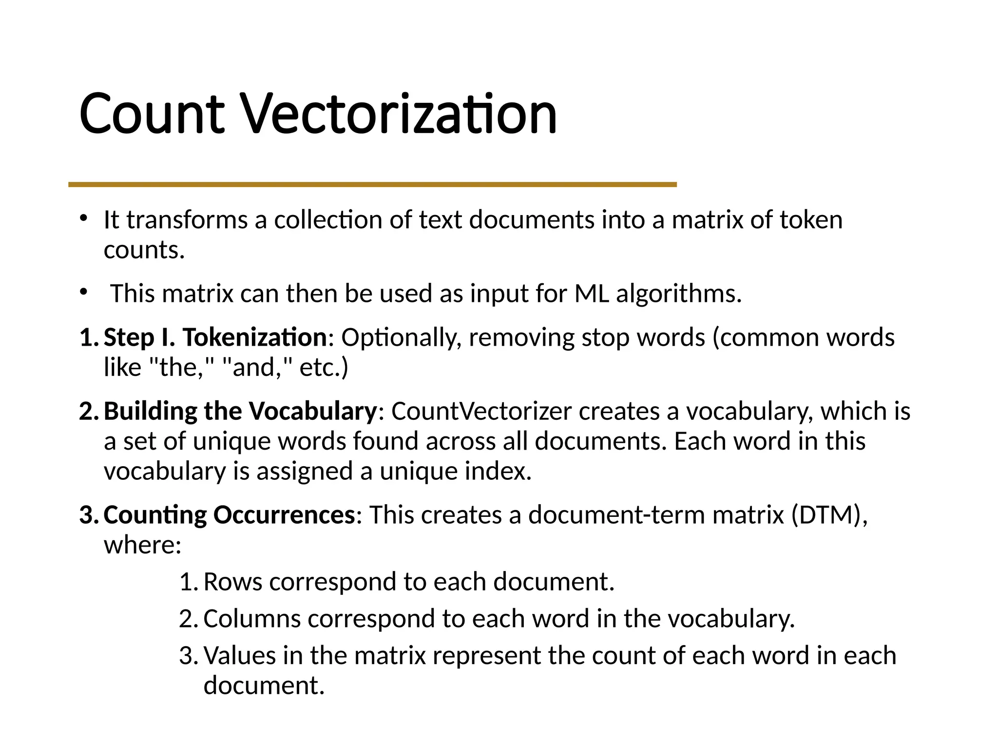
CountVectorize
Docum
ent
code fun iis love progra
mming
to
0 0 0 1 0 1 1 0
1 0 1 0 1 0 1 0
2 1 0 1 0 1 0 1
Step 3: Creating Document-Term Matrix
The document-term matrix would look like this:
5.
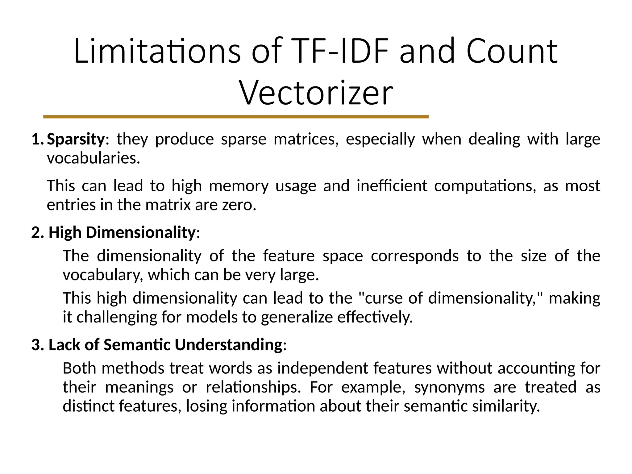
Limitations of TF-IDFand Count
Vectorizer
1.Sparsity: they produce sparse matrices, especially when dealing with large
vocabularies.
This can lead to high memory usage and inefficient computations, as most
entries in the matrix are zero.
2. High Dimensionality:
The dimensionality of the feature space corresponds to the size of the
vocabulary, which can be very large.
This high dimensionality can lead to the "curse of dimensionality," making
it challenging for models to generalize effectively.
3. Lack of Semantic Understanding:
Both methods treat words as independent features without accounting for
their meanings or relationships. For example, synonyms are treated as
distinct features, losing information about their semantic similarity.
6.
Limitations of TF-IDFand
CountVectorizer
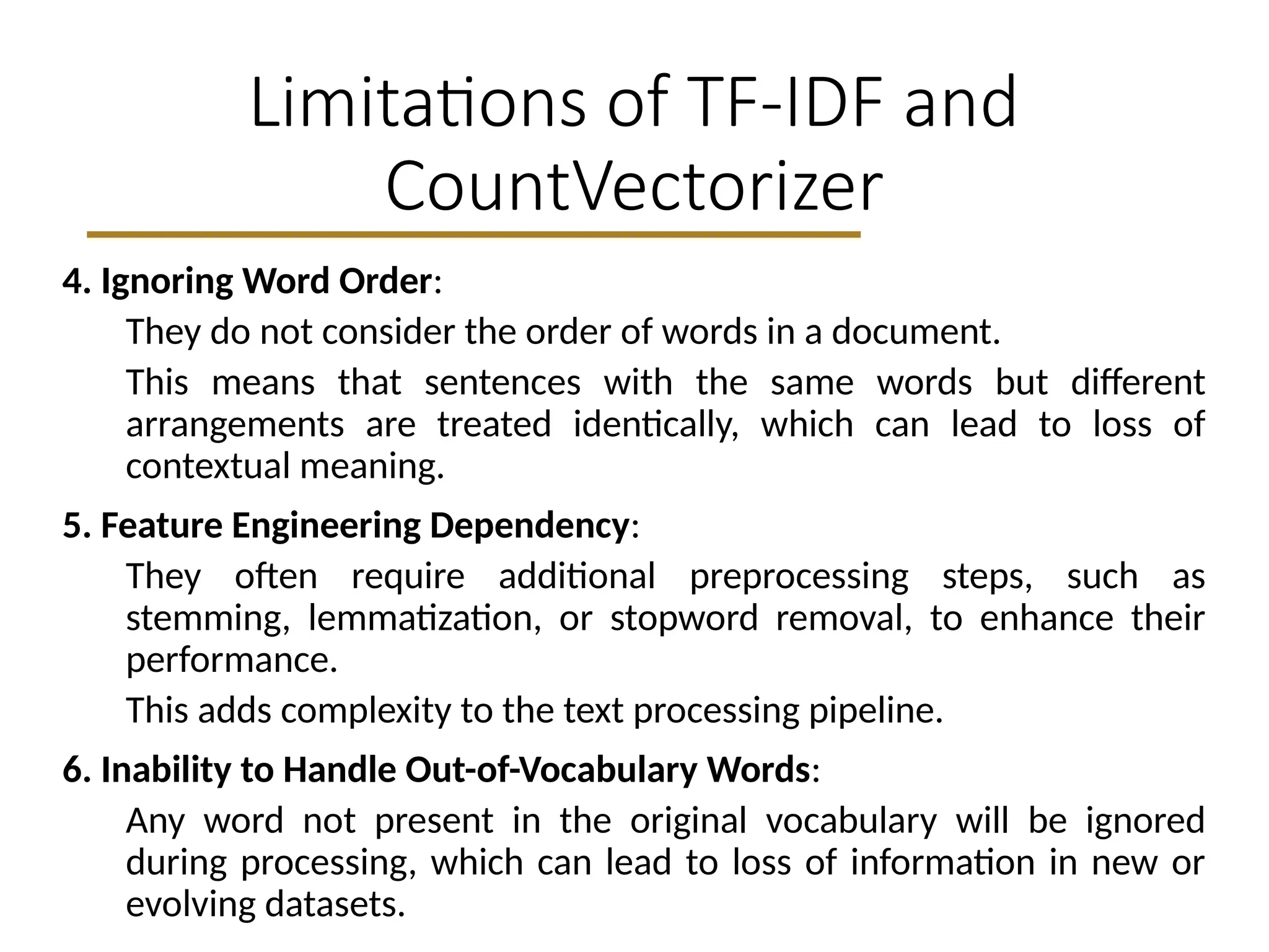
4. Ignoring Word Order:
They do not consider the order of words in a document.
This means that sentences with the same words but different
arrangements are treated identically, which can lead to loss of
contextual meaning.
5. Feature Engineering Dependency:
They often require additional preprocessing steps, such as
stemming, lemmatization, or stopword removal, to enhance their
performance.
This adds complexity to the text processing pipeline.
6. Inability to Handle Out-of-Vocabulary Words:
Any word not present in the original vocabulary will be ignored
during processing, which can lead to loss of information in new or
evolving datasets.
7.
Word embeddings
• Idea:learn an embedding from words into vectors
• Need to have a function W(word) that returns a
vector encoding that word.
8.
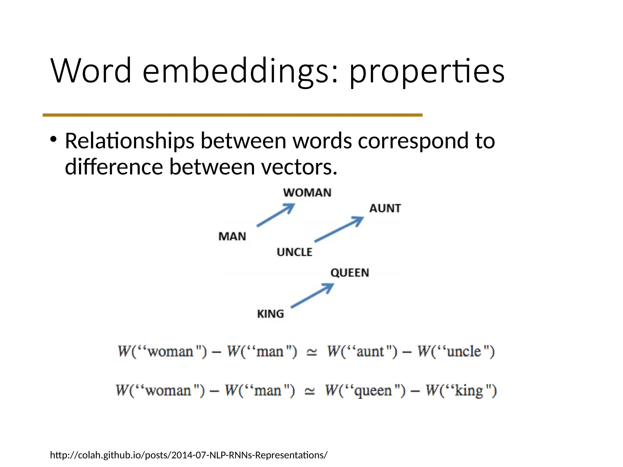
Word embeddings: properties
•Relationships between words correspond to
difference between vectors.
http://colah.github.io/posts/2014-07-NLP-RNNs-Representations/
9.
Word embeddings: questions
•How big should the embedding space be?
• Trade-offs like any other machine learning problem –
greater capacity versus efficiency and overfitting.
• How do we find W?
• Often as part of a prediction or classification task
involving neighboring words.
10.
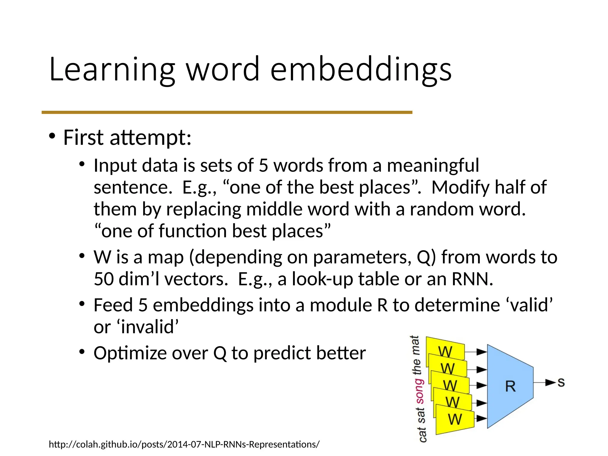
Learning word embeddings
•First attempt:
• Input data is sets of 5 words from a meaningful
sentence. E.g., “one of the best places”. Modify half of
them by replacing middle word with a random word.
“one of function best places”
• W is a map (depending on parameters, Q) from words to
50 dim’l vectors. E.g., a look-up table or an RNN.
• Feed 5 embeddings into a module R to determine ‘valid’
or ‘invalid’
• Optimize over Q to predict better
http://colah.github.io/posts/2014-07-NLP-RNNs-Representations/
11.
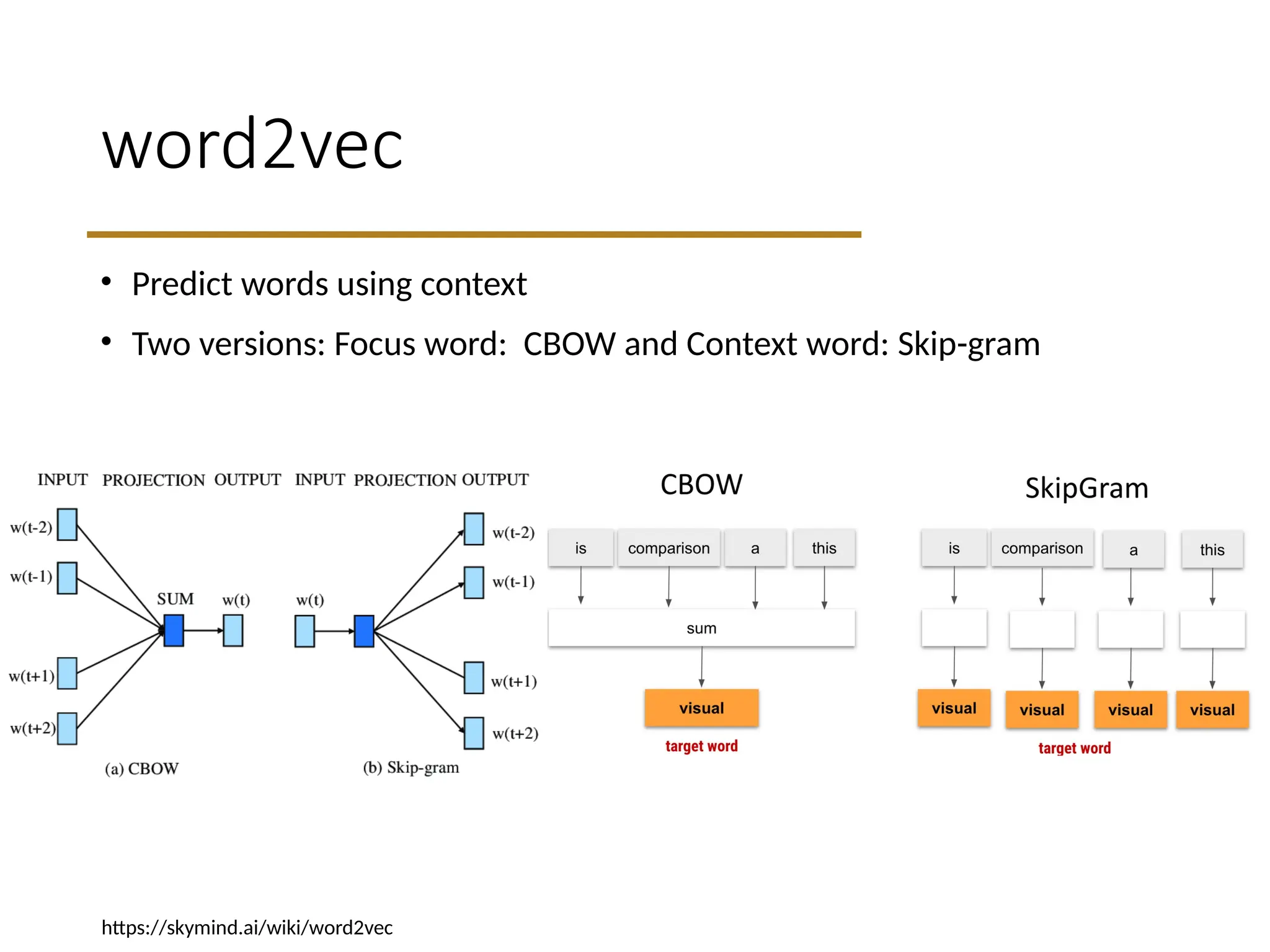
word2vec
• Predict wordsusing context
• Two versions: Focus word: CBOW and Context word: Skip-gram
https://skymind.ai/wiki/word2vec
12.
CBOW
• Bag ofwords
• Gets rid of word order. Used in discrete case using counts of words
that appear.
• CBOW
• Takes vector embeddings of n words before target and n words
after and adds them (as vectors).
• Also removes word order, but the vector sum is meaningful enough
to deduce missing word.
13.
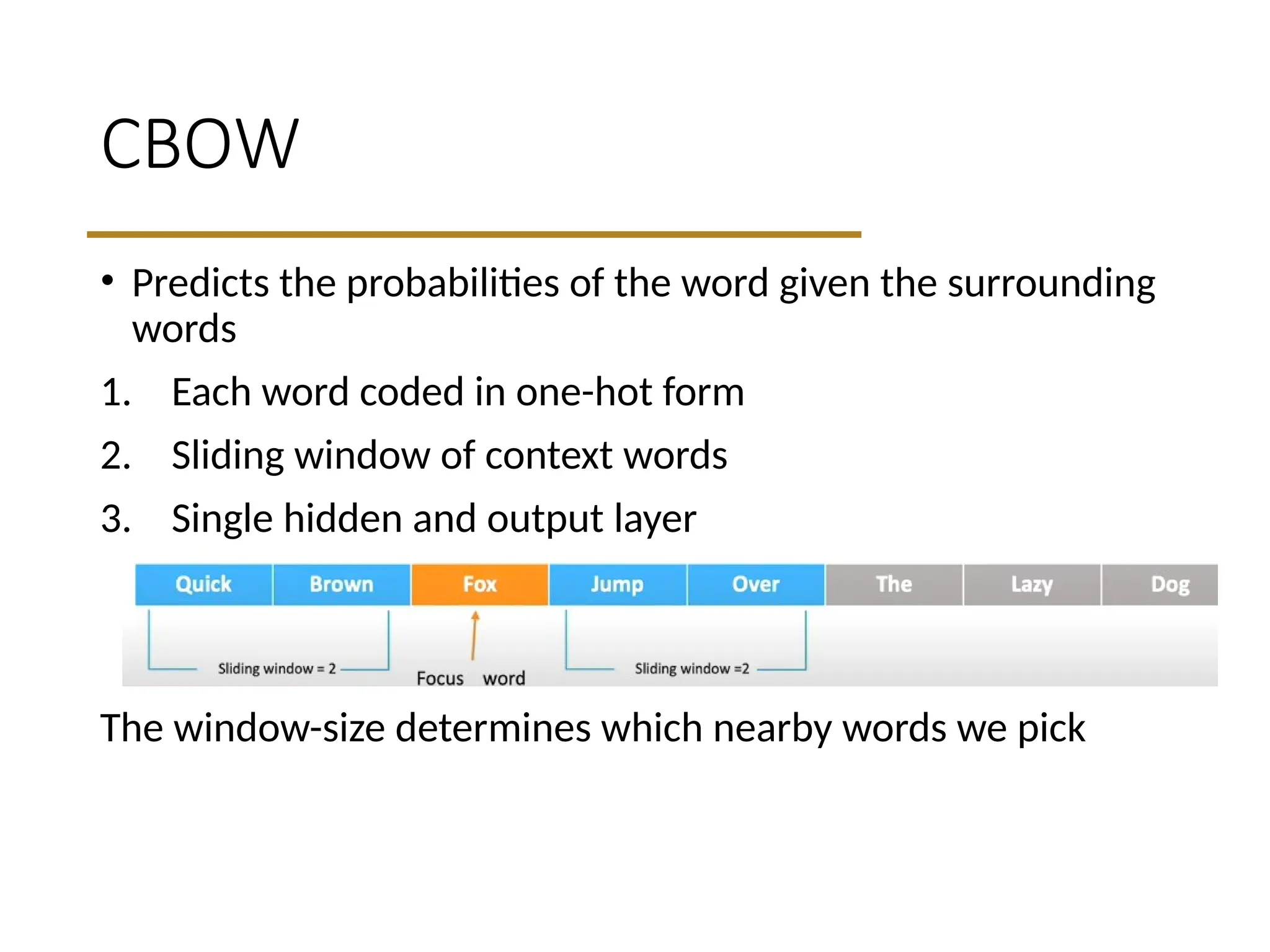
CBOW
• Predicts theprobabilities of the word given the surrounding
words
1. Each word coded in one-hot form
2. Sliding window of context words
3. Single hidden and output layer
The window-size determines which nearby words we pick
14.
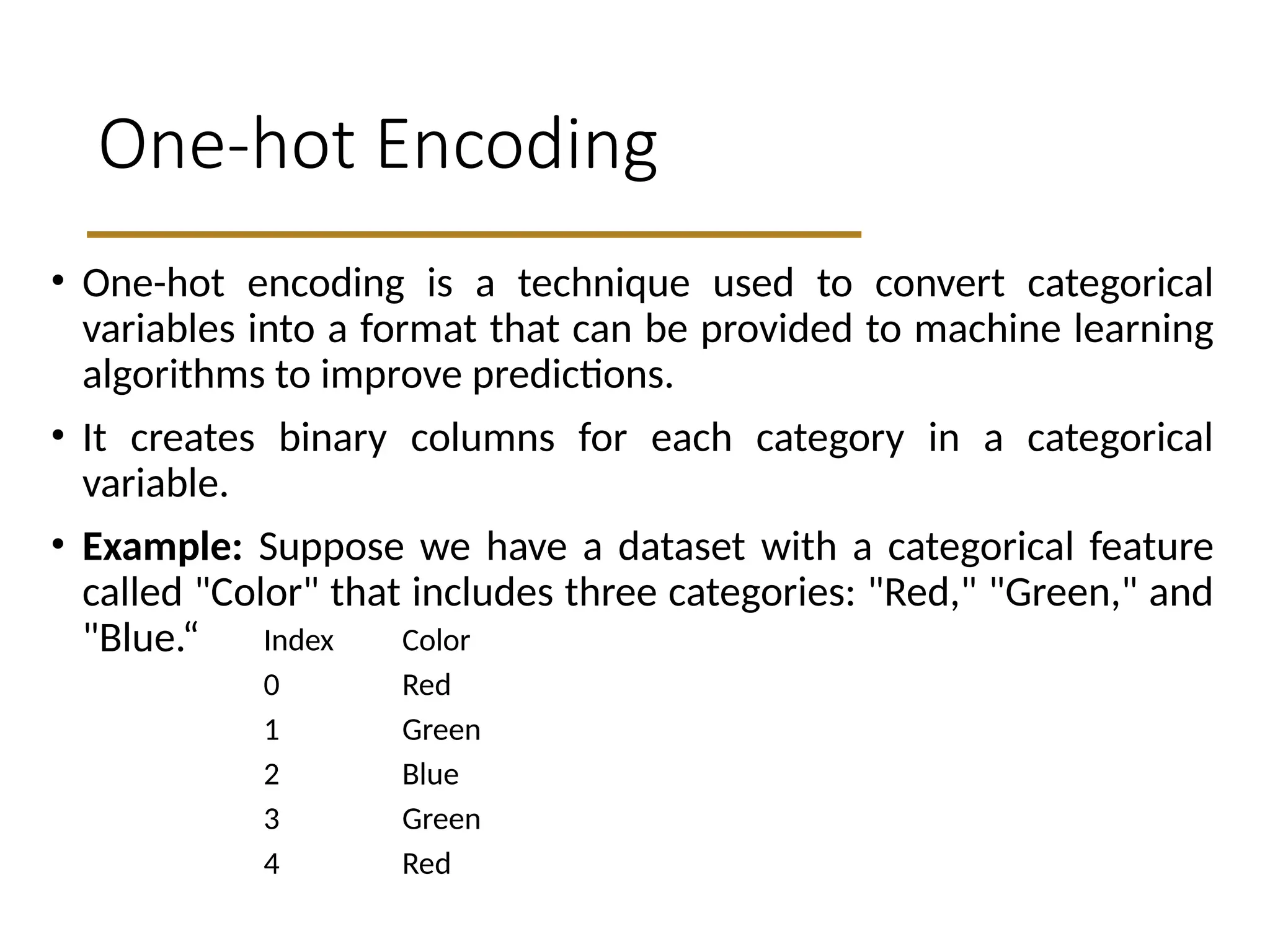
One-hot Encoding
• One-hotencoding is a technique used to convert categorical
variables into a format that can be provided to machine learning
algorithms to improve predictions.
• It creates binary columns for each category in a categorical
variable.
• Example: Suppose we have a dataset with a categorical feature
called "Color" that includes three categories: "Red," "Green," and
"Blue.“ Index Color
0 Red
1 Green
2 Blue
3 Green
4 Red
15.
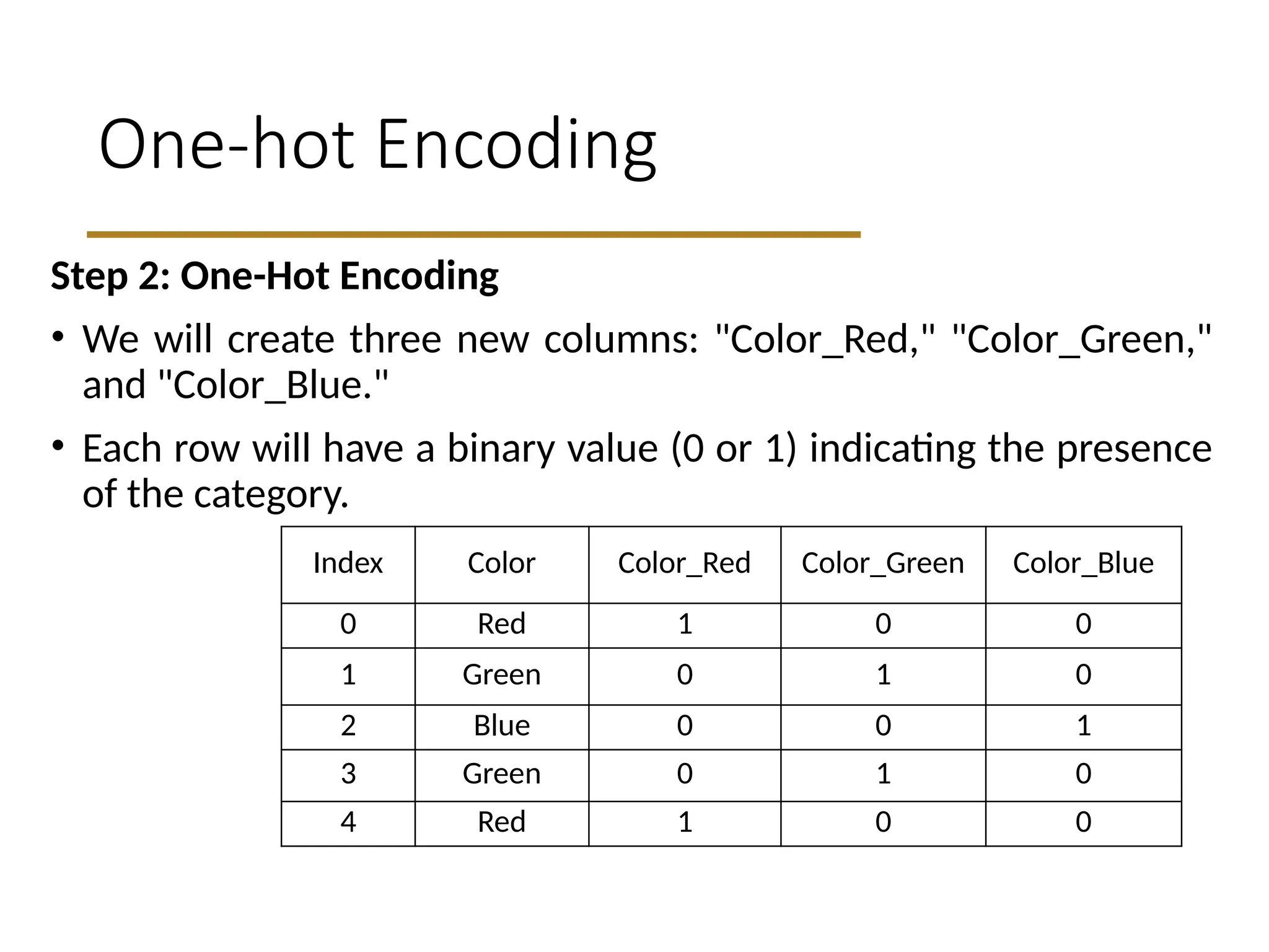
One-hot Encoding
Step 2:One-Hot Encoding
• We will create three new columns: "Color_Red," "Color_Green,"
and "Color_Blue."
• Each row will have a binary value (0 or 1) indicating the presence
of the category.
Index Color Color_Red Color_Green Color_Blue
0 Red 1 0 0
1 Green 0 1 0
2 Blue 0 0 1
3 Green 0 1 0
4 Red 1 0 0
16.
Benefits
1.No Ordinality: One-hotencoding helps to avoid any ordinal
relationship between categories.
2.Compatibility: Makes the data compatible with machine learning
algorithms that assume numerical input.
import pandas as pd
# Create a Data
Framedata = {'Color': ['Red', 'Green', 'Blue', 'Green', 'Red’]}
df = pd.Data
Frame(data)
# One-hot encode the 'Color' column
one_hot_encoded_df = pd.get_dummies(df,
columns=['Color'])print(one_hot_encoded_df)
17.
High-cardinality categories
• Whendealing with many categorical values (high cardinality), l encoding
methods like one-hot encoding can lead to a significant increase in
dimensionality, which may cause issues such as:
1.Curse of Dimensionality: More features can lead to overfitting,
especially with limited data.
2.Increased Computational Cost: More features require more memory
and computational power, slowing down model training and inference.
18.
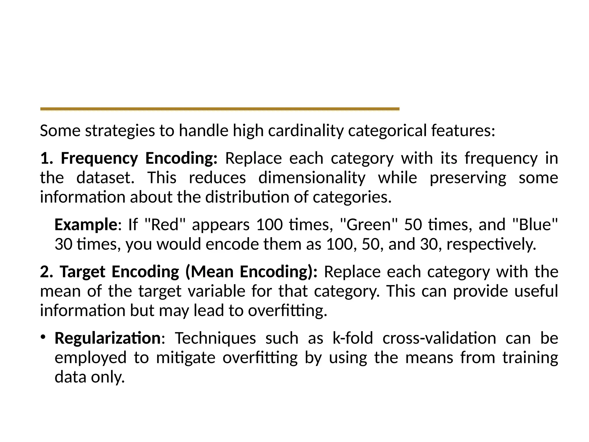
Some strategies tohandle high cardinality categorical features:
1. Frequency Encoding: Replace each category with its frequency in
the dataset. This reduces dimensionality while preserving some
information about the distribution of categories.
Example: If "Red" appears 100 times, "Green" 50 times, and "Blue"
30 times, you would encode them as 100, 50, and 30, respectively.
2. Target Encoding (Mean Encoding): Replace each category with the
mean of the target variable for that category. This can provide useful
information but may lead to overfitting.
• Regularization: Techniques such as k-fold cross-validation can be
employed to mitigate overfitting by using the means from training
data only.
19.
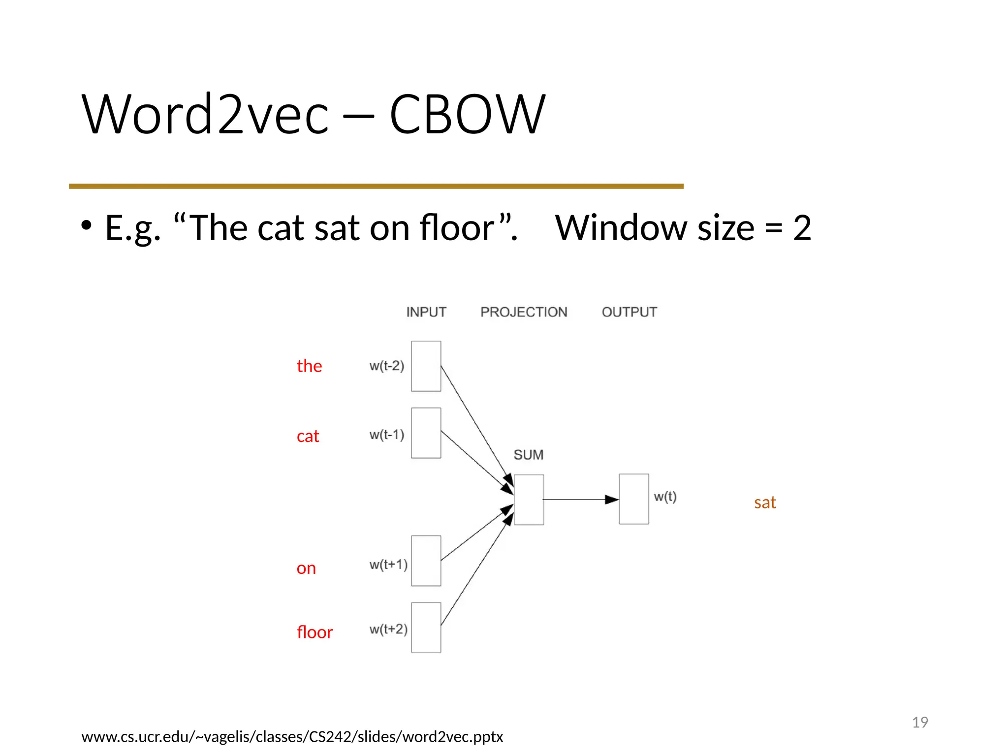
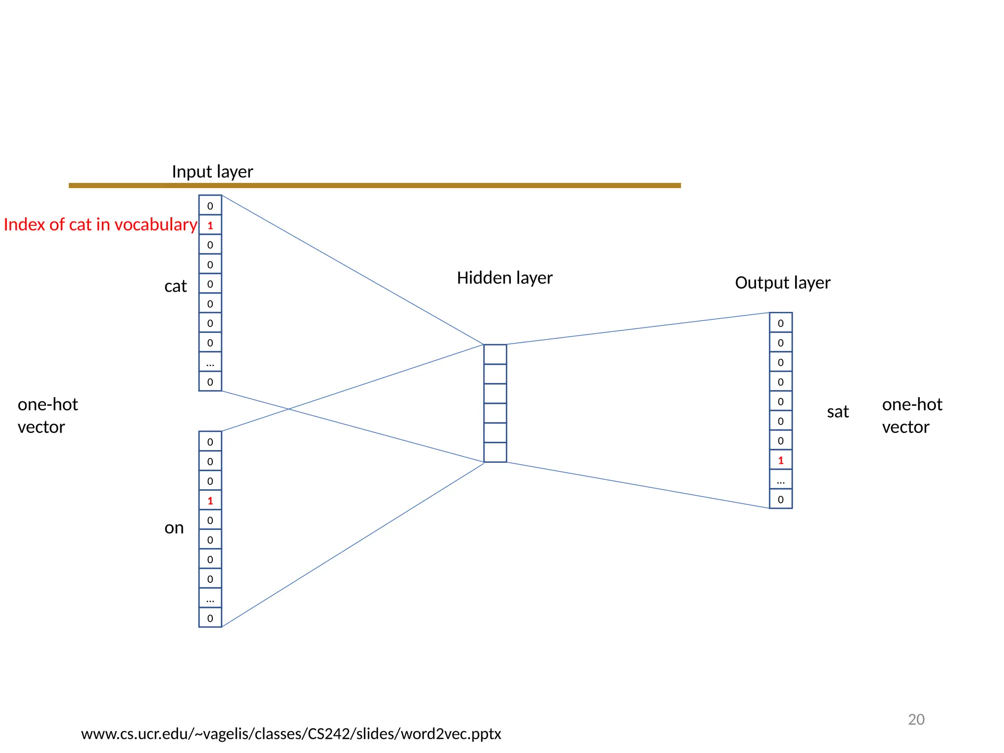
Word2vec – CBOW
•E.g. “The cat sat on floor”. Window size = 2
19
the
cat
on
floor
sat
www.cs.ucr.edu/~vagelis/classes/CS242/slides/word2vec.pptx
21
0
1
0
0
0
0
0
0
…
0
0
0
0
1
0
0
0
0
…
0
cat
on
0
0
0
0
0
0
0
1
…
0
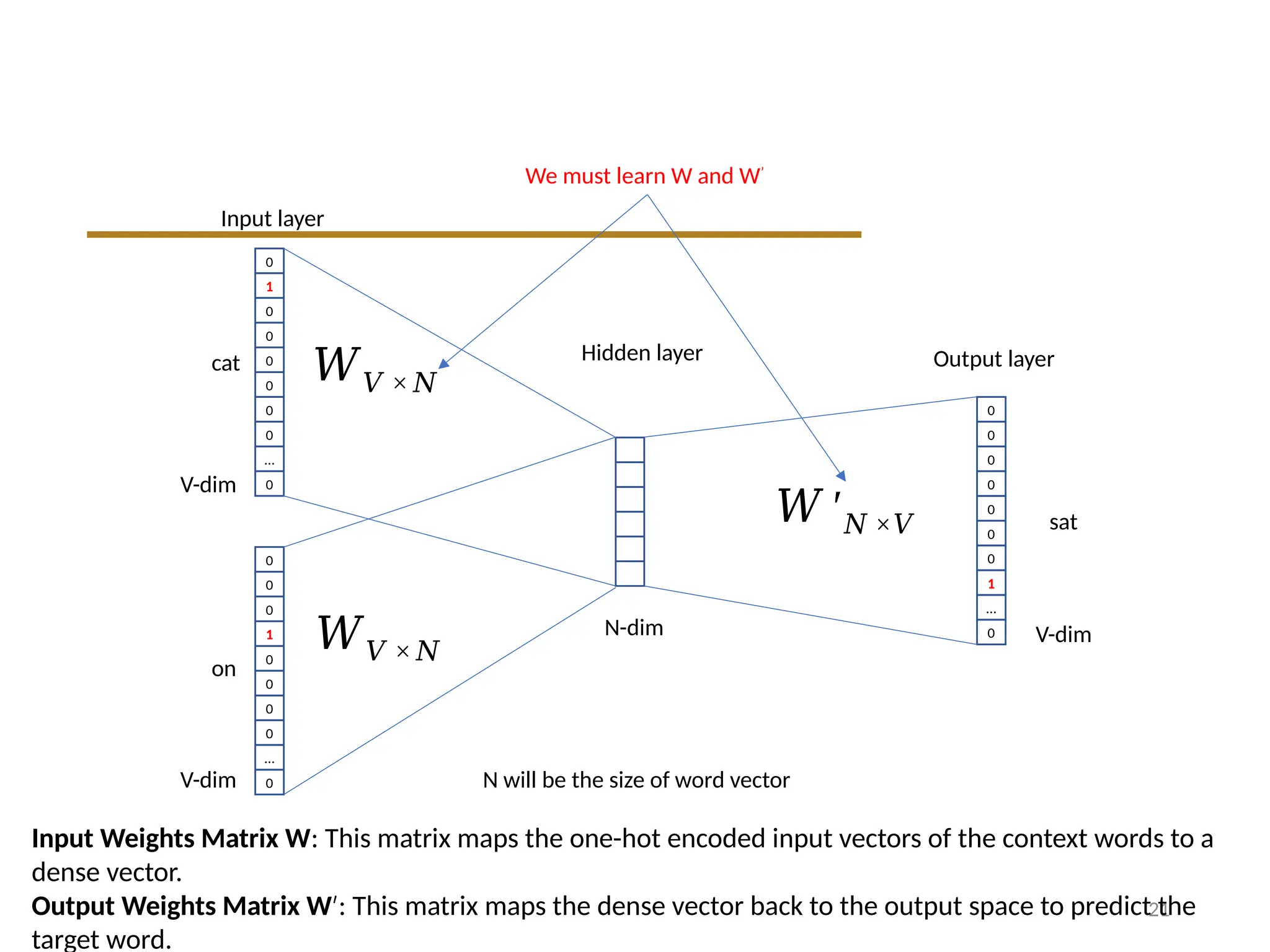
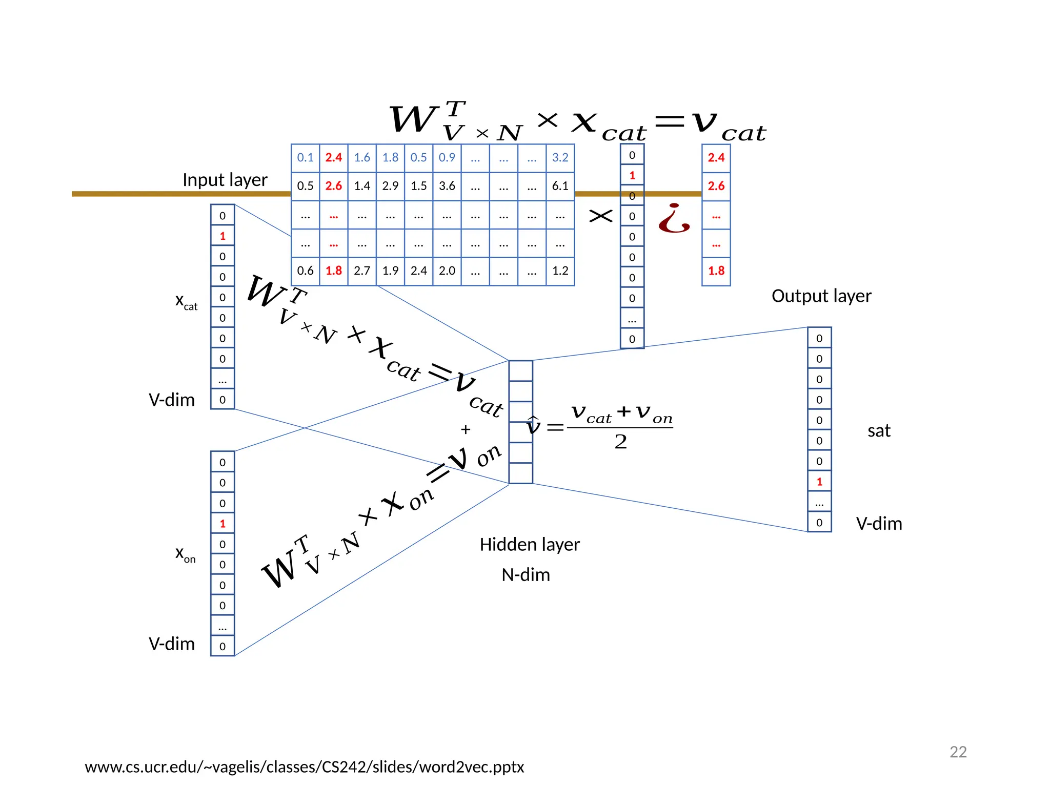
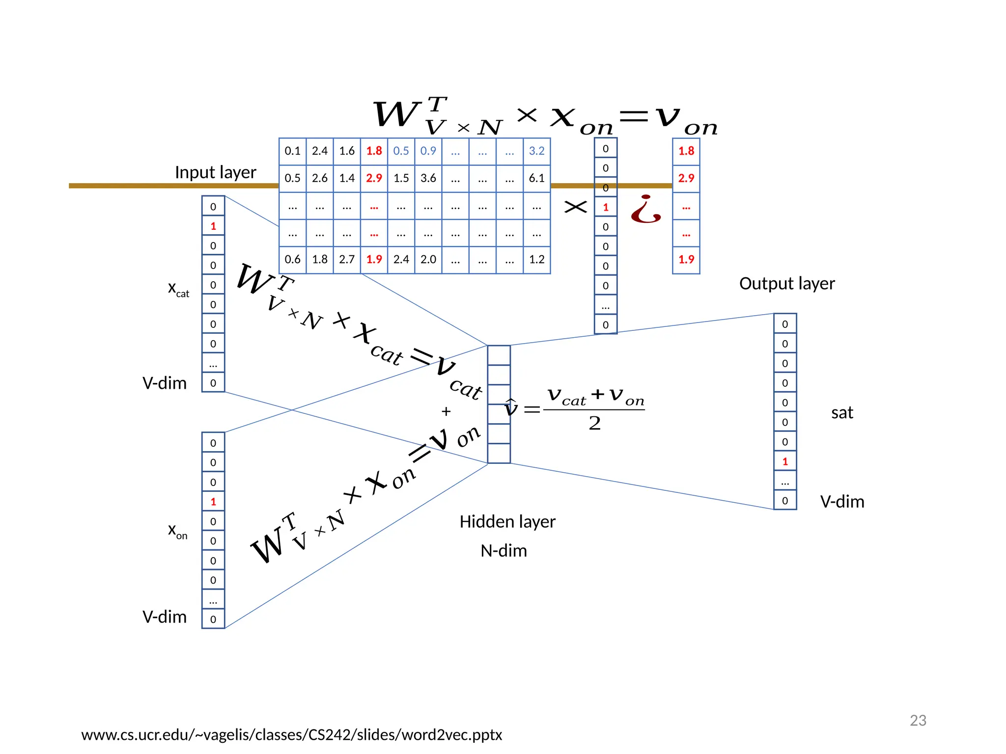
Input layer
Hidden layer
sat
Outputlayer
𝑊𝑉 × 𝑁
𝑊𝑉 × 𝑁
V-dim
V-dim
N-dim
𝑊 ′𝑁 ×𝑉
V-dim
N will be the size of word vector
We must learn W and W’
Input Weights Matrix W: This matrix maps the one-hot encoded input vectors of the context words to a
dense vector.
Output Weights Matrix W′: This matrix maps the dense vector back to the output space to predict the
target word.
24
0
1
0
0
0
0
0
0
…
0
0
0
0
1
0
0
0
0
…
0
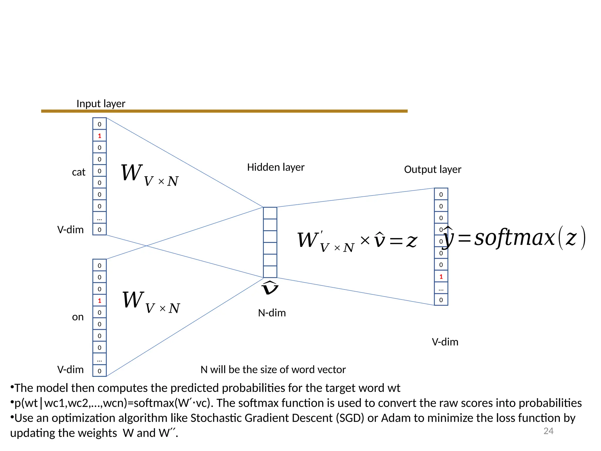
cat
on
0
0
0
0
0
0
0
1
…
0
Input layer
Hidden layerOutput layer
𝑊𝑉 × 𝑁
𝑊𝑉 × 𝑁
V-dim
V-dim
N-dim
𝑊𝑉 × 𝑁
′
×^
𝑣=𝑧
V-dim
N will be the size of word vector
^
𝑣
^
𝑦=𝑠𝑜𝑓𝑡𝑚𝑎𝑥(𝑧)
•The model then computes the predicted probabilities for the target word wt
•p(wt wc1,wc2,…,wcn)=softmax(W vc). The softmax function is used to convert the raw scores into probabilities
∣ ′⋅
•Use an optimization algorithm like Stochastic Gradient Descent (SGD) or Adam to minimize the loss function by
updating the weights W and W .
′′
26
0
1
0
0
0
0
0
0
…
0
0
0
0
1
0
0
0
0
…
0
xcat
xon
0
0
0
0
0
0
0
1
…
0
Input layer
Hidden layer
sat
Outputlayer
V-dim
V-dim
N-dim
V-dim
𝑊𝑉 ×𝑁
❑
𝑊𝑉 × 𝑁
❑
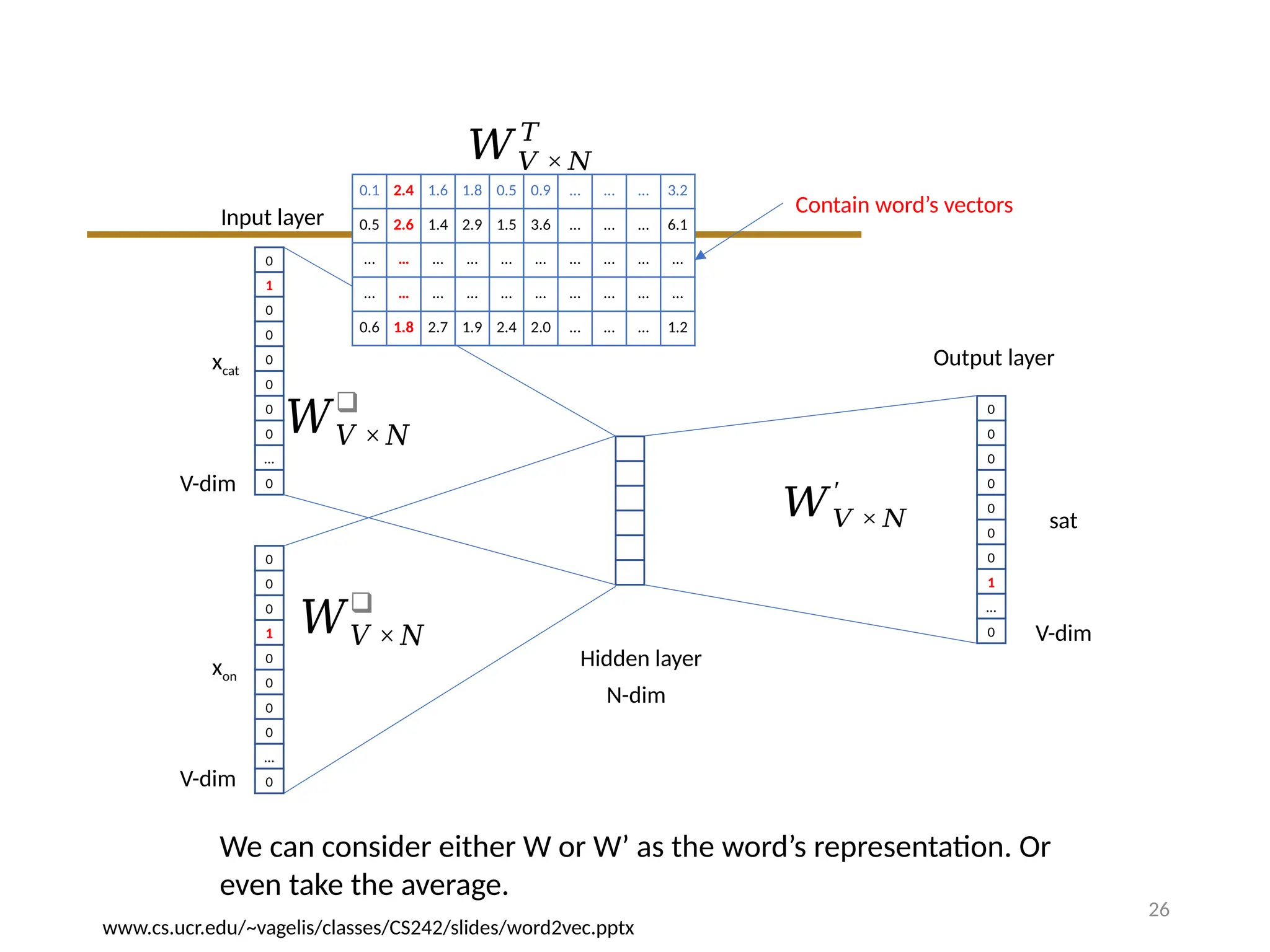
0.1 2.4 1.6 1.8 0.5 0.9 … … … 3.2
0.5 2.6 1.4 2.9 1.5 3.6 … … … 6.1
… … … … … … … … … …
… … … … … … … … … …
0.6 1.8 2.7 1.9 2.4 2.0 … … … 1.2
𝑊𝑉 × 𝑁
𝑇
Contain word’s vectors
𝑊𝑉 × 𝑁
′
We can consider either W or W’ as the word’s representation. Or
even take the average.
www.cs.ucr.edu/~vagelis/classes/CS242/slides/word2vec.pptx
27.
Example Calculation
• Given:
•Vocabulary: { "cat", "dog", "sat", "on", "the" }
• Target word: "sat"
• Context window size: 1
• Context words: "the", "cat"
• Step 1: One-Hot Encoding
• Assuming "sat" is at index 2:
• One-hot vector for "the": [0, 0, 0, 0, 1]
• One-hot vector for "cat": [0, 1, 0, 0, 0]
28.
Step 2: WeightMatrices
• Assume N=3 (embedding size), with Input Weight W:
[[0.1, 0.2, 0.3], # cat
[0.4, 0.5, 0.6], # dog
[0.7, 0.8, 0.9], # sat
[0.1, 0.4, 0.2], # on
[0.3, 0.5, 0.7]] # the
[[0.1, 0.2, 0.3, 0.4, 0.5], # cat
[0.6, 0.7, 0.8, 0.9, 0.1], # dog
[0.2, 0.3, 0.4, 0.5, 0.6], # sat
[0.1, 0.2, 0.3, 0.4, 0.5], # on
[0.6, 0.7, 0.8, 0.9, 0.1]] # the
Output Weight W′
29.
• Step 3:Compute Dense Vector for Context For context
words "the" and "cat":
• Calculate their dense vectors:
• For "the":𝑣 =
𝑡ℎ𝑒 𝑊𝑇 _ (" ")=[0.3,0.5,0.7]
⋅𝑜𝑛𝑒 ℎ𝑜𝑡 𝑡ℎ𝑒
• For "cat":𝑣 =
𝑐𝑎𝑡 𝑊𝑇 _ (" ")=[0.1,0.2,0.3
⋅𝑜𝑛𝑒 ℎ𝑜𝑡 𝑐𝑎𝑡
• Average the dense vectors:
𝑣𝑐=1/2( + )=1/2([0.3,0.5,0.7]+[0.1,0.2,0.3])
𝑣𝑡ℎ𝑒 𝑣𝑐𝑎𝑡
30.
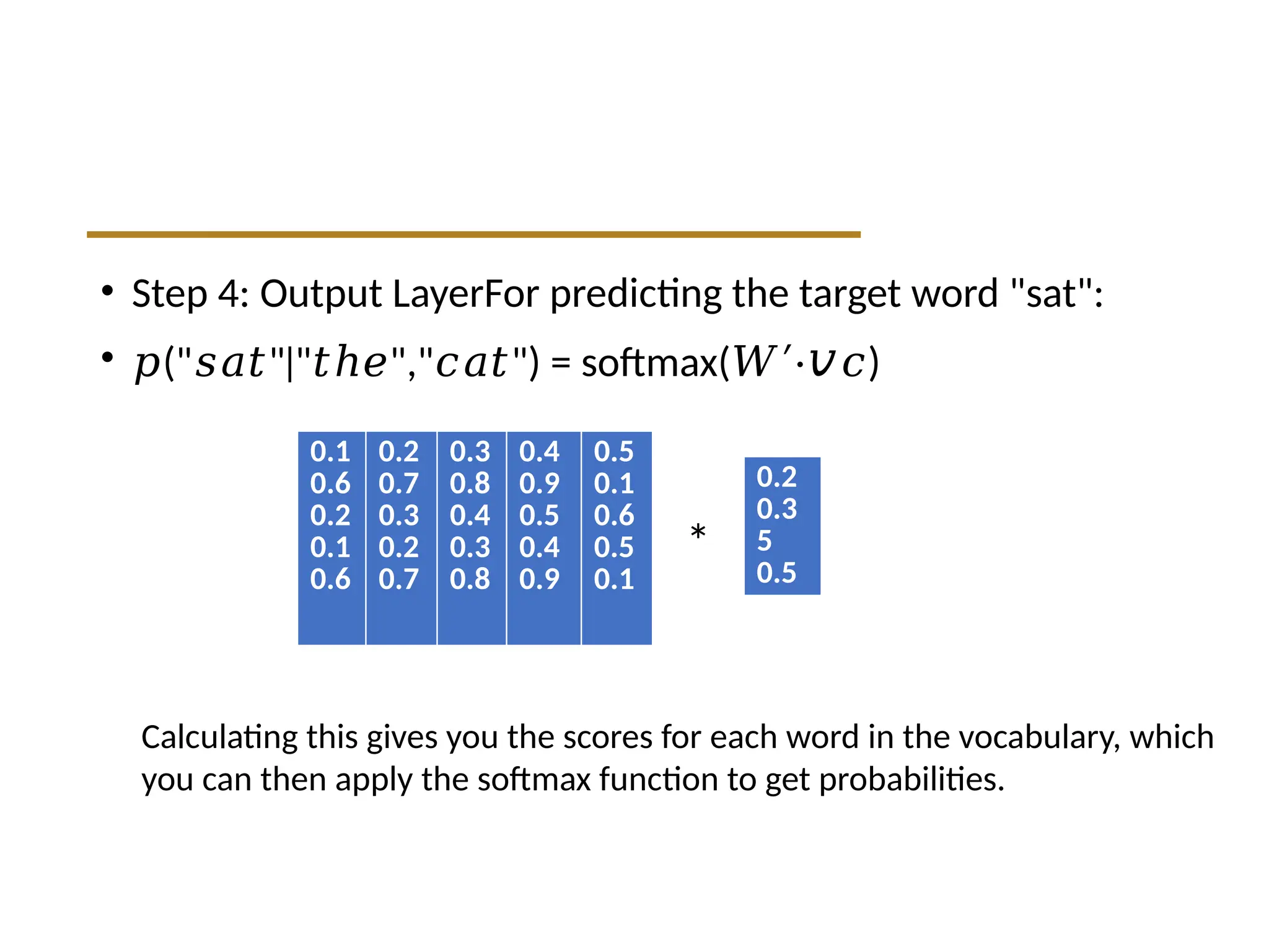
• Step 4:Output LayerFor predicting the target word "sat":
• 𝑝(" " " "," ") = softmax(
𝑠𝑎𝑡 ∣ 𝑡ℎ𝑒 𝑐𝑎𝑡 𝑊′⋅𝑣 )
𝑐
0.1
0.6
0.2
0.1
0.6
0.2
0.7
0.3
0.2
0.7
0.3
0.8
0.4
0.3
0.8
0.4
0.9
0.5
0.4
0.9
0.5
0.1
0.6
0.5
0.1
0.2
0.3
5
0.5
Calculating this gives you the scores for each word in the vocabulary, which
you can then apply the softmax function to get probabilities.
*
31.
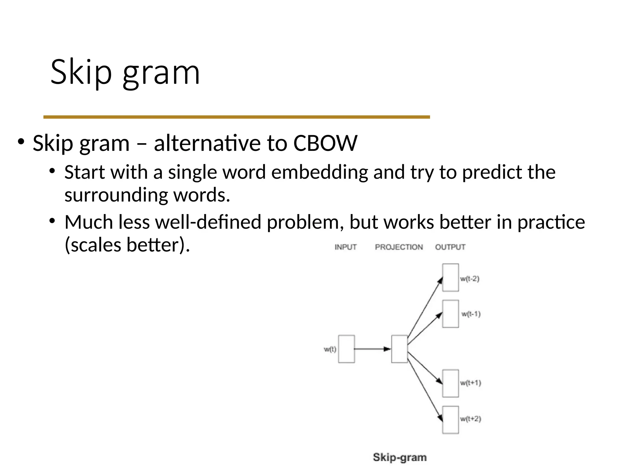
Skip gram
• Skipgram – alternative to CBOW
• Start with a single word embedding and try to predict the
surrounding words.
• Much less well-defined problem, but works better in practice
(scales better).
32.
Skip gram
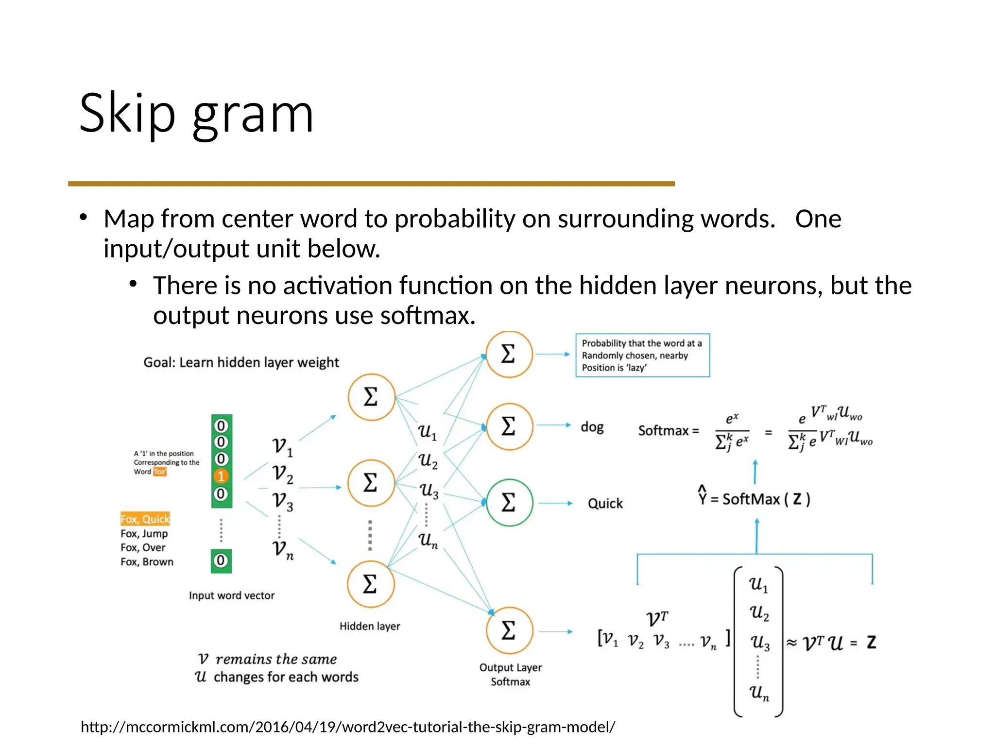
• Mapfrom center word to probability on surrounding words. One
input/output unit below.
• There is no activation function on the hidden layer neurons, but the
output neurons use softmax.
http://mccormickml.com/2016/04/19/word2vec-tutorial-the-skip-gram-model/
33.
Skip gram example
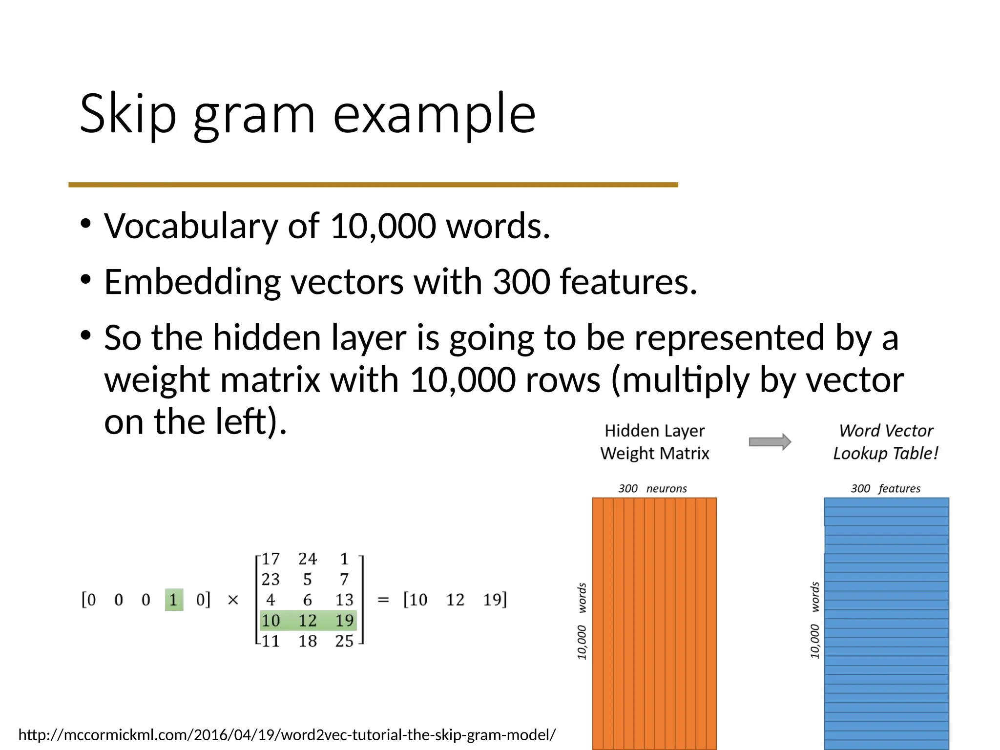
•Vocabulary of 10,000 words.
• Embedding vectors with 300 features.
• So the hidden layer is going to be represented by a
weight matrix with 10,000 rows (multiply by vector
on the left).
http://mccormickml.com/2016/04/19/word2vec-tutorial-the-skip-gram-model/
1. Word Vectors
•Each word in the vocabulary has a corresponding vector of numbers. For
example, a word vector might look like `[0.1, 0.2, -0.3, ...]`.
• The length of these vectors is determined by the `vector_size` parameter (in this
case, 10). This means each word is represented in a 10-dimensional space.
2. Semantic Meaning:
• The values in the vectors represent the position of the words in the embedding
space. Words with similar meanings or that appear in similar contexts will have
vectors that are close to each other in this space.
• For instance, if "cat" and "dog" are both pets and often appear in similar
contexts, their vectors will be similar, indicating a relationship.
3. Dimensionality:
• The dimensionality of the vectors (e.g., 10) is a hyperparameter that can be
tuned. Higher dimensions can capture more information but may also lead to
overfitting and increased computational costs.
• - Lower dimensions may result in loss of information but can be more efficient.
37.
4. Training Process:
•- The embeddings are learned through a process where the model adjusts
the vector representations based on the context of words in the training
sentences.
• - In CBOW, the model uses surrounding words (context) to predict the target
word. In contrast, Skip-Gram does the opposite by using a target word to
predict its context.
5. Applications of Word Vectors:
• Similarity Measurement: You can calculate the cosine similarity between
word vectors to find similar words. For example,
`cosine_similarity(cbow_model.wv['cat'], cbow_model.wv['dog'])` could yield
a value close to 1, indicating similarity.
• Analogy Tasks: Word vectors can be used in analogy tasks (e.g., "king - man +
woman = queen"), where vector arithmetic reveals relationships between
words.
38.
Each word willhave a corresponding vector of specified size (in this
case, 10).
Example vector representation
• CBOW Vector for 'cat': [ 0.01, -0.02, 0.03, ...]
• Skip-Gram Vector for 'cat': [ 0.02, -0.01, 0.04, ...]
• Similar words to 'cat' in CBOW: [('the', 0.56), ('sat', 0.45), ('dog',
0.40)]
• Similar words to 'cat' in Skip-Gram: [('the', 0.58), ('sat', 0.43), ('dog',
0.39)]
39.
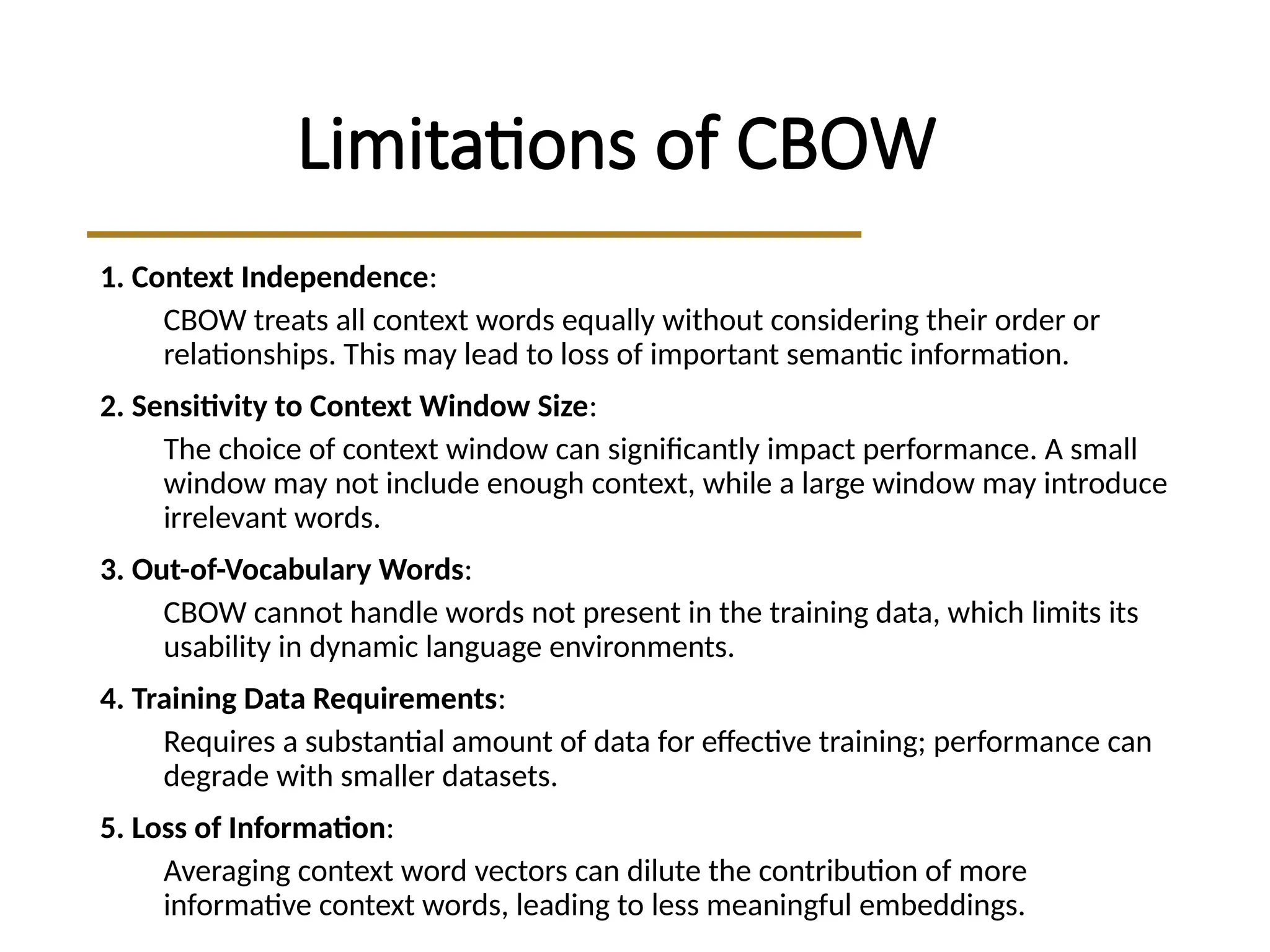
Limitations of CBOW
1.Context Independence:
CBOW treats all context words equally without considering their order or
relationships. This may lead to loss of important semantic information.
2. Sensitivity to Context Window Size:
The choice of context window can significantly impact performance. A small
window may not include enough context, while a large window may introduce
irrelevant words.
3. Out-of-Vocabulary Words:
CBOW cannot handle words not present in the training data, which limits its
usability in dynamic language environments.
4. Training Data Requirements:
Requires a substantial amount of data for effective training; performance can
degrade with smaller datasets.
5. Loss of Information:
Averaging context word vectors can dilute the contribution of more
informative context words, leading to less meaningful embeddings.
40.
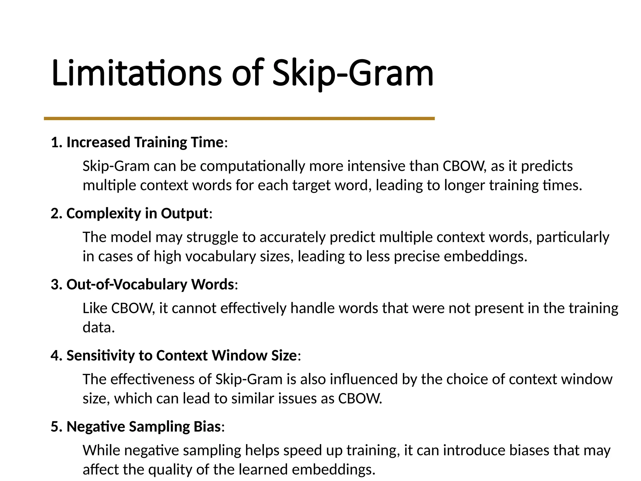
Limitations of Skip-Gram
1.Increased Training Time:
Skip-Gram can be computationally more intensive than CBOW, as it predicts
multiple context words for each target word, leading to longer training times.
2. Complexity in Output:
The model may struggle to accurately predict multiple context words, particularly
in cases of high vocabulary sizes, leading to less precise embeddings.
3. Out-of-Vocabulary Words:
Like CBOW, it cannot effectively handle words that were not present in the training
data.
4. Sensitivity to Context Window Size:
The effectiveness of Skip-Gram is also influenced by the choice of context window
size, which can lead to similar issues as CBOW.
5. Negative Sampling Bias:
While negative sampling helps speed up training, it can introduce biases that may
affect the quality of the learned embeddings.
41.
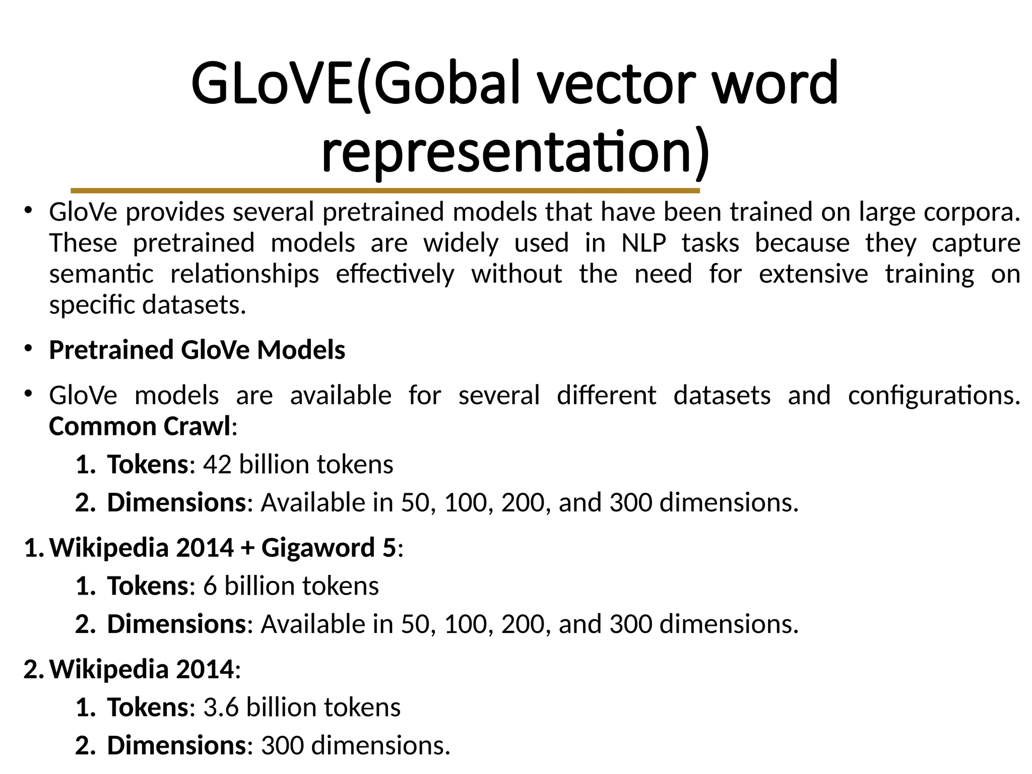
GLoVE(Gobal vector word
representation)
•GloVe provides several pretrained models that have been trained on large corpora.
These pretrained models are widely used in NLP tasks because they capture
semantic relationships effectively without the need for extensive training on
specific datasets.
• Pretrained GloVe Models
• GloVe models are available for several different datasets and configurations.
Common Crawl:
1. Tokens: 42 billion tokens
2. Dimensions: Available in 50, 100, 200, and 300 dimensions.
1.Wikipedia 2014 + Gigaword 5:
1. Tokens: 6 billion tokens
2. Dimensions: Available in 50, 100, 200, and 300 dimensions.
2.Wikipedia 2014:
1. Tokens: 3.6 billion tokens
2. Dimensions: 300 dimensions.
42.
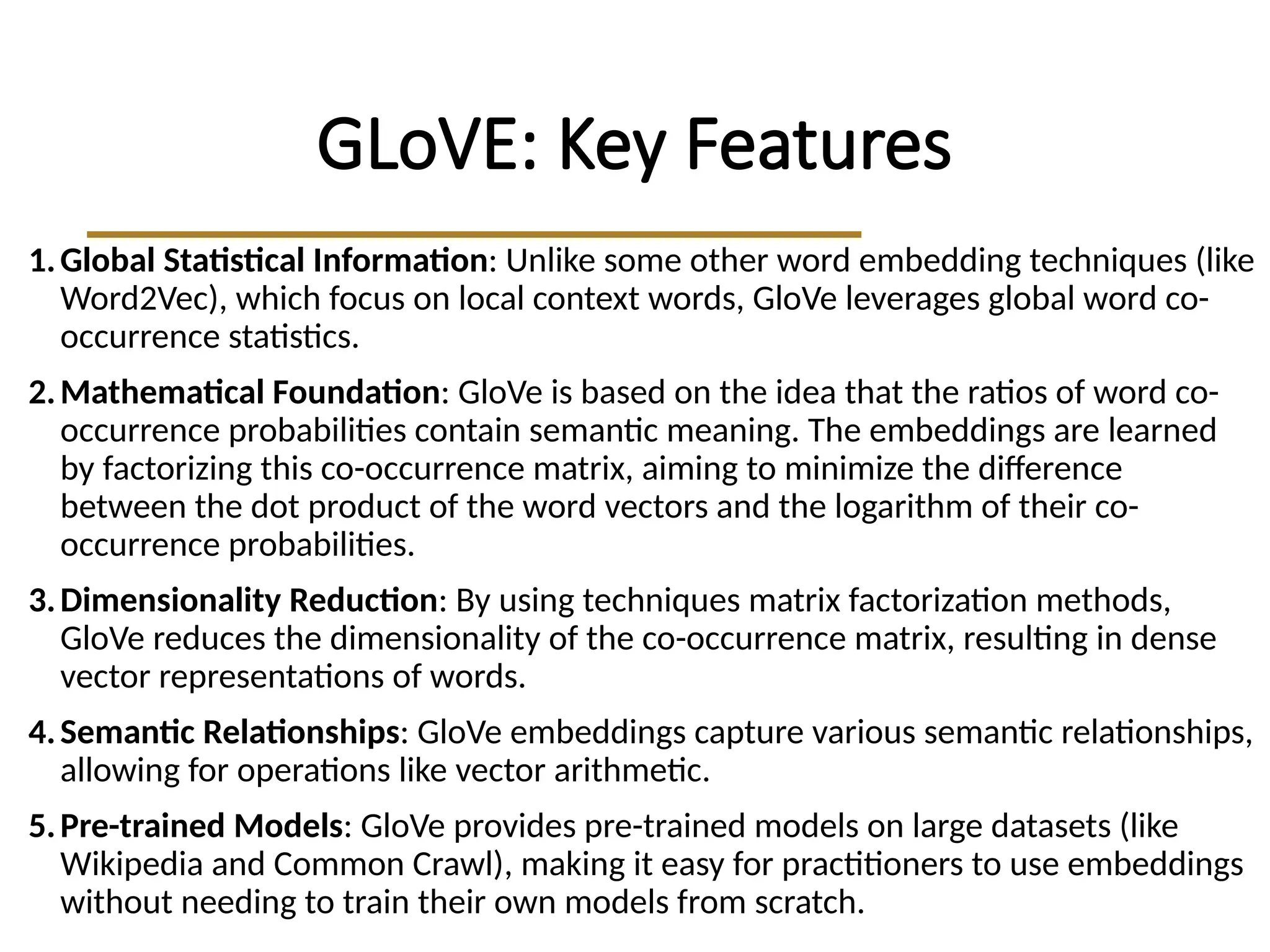
GLoVE: Key Features
1.GlobalStatistical Information: Unlike some other word embedding techniques (like
Word2Vec), which focus on local context words, GloVe leverages global word co-
occurrence statistics.
2.Mathematical Foundation: GloVe is based on the idea that the ratios of word co-
occurrence probabilities contain semantic meaning. The embeddings are learned
by factorizing this co-occurrence matrix, aiming to minimize the difference
between the dot product of the word vectors and the logarithm of their co-
occurrence probabilities.
3.Dimensionality Reduction: By using techniques matrix factorization methods,
GloVe reduces the dimensionality of the co-occurrence matrix, resulting in dense
vector representations of words.
4.Semantic Relationships: GloVe embeddings capture various semantic relationships,
allowing for operations like vector arithmetic.
5.Pre-trained Models: GloVe provides pre-trained models on large datasets (like
Wikipedia and Common Crawl), making it easy for practitioners to use embeddings
without needing to train their own models from scratch.
43.
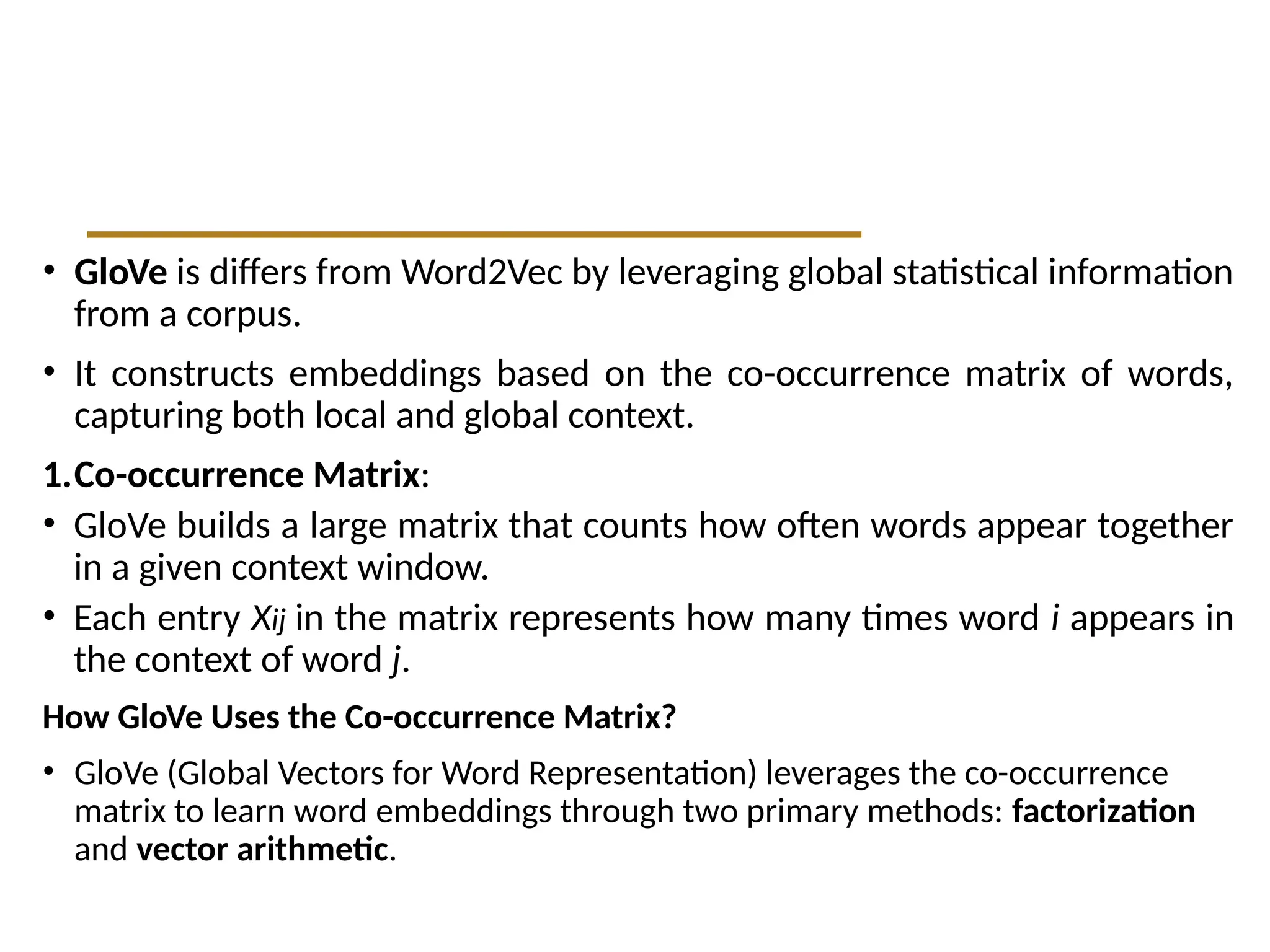
• GloVe isdiffers from Word2Vec by leveraging global statistical information
from a corpus.
• It constructs embeddings based on the co-occurrence matrix of words,
capturing both local and global context.
1.Co-occurrence Matrix:
• GloVe builds a large matrix that counts how often words appear together
in a given context window.
• Each entry Xij in the matrix represents how many times word i appears in
the context of word j.
How GloVe Uses the Co-occurrence Matrix?
• GloVe (Global Vectors for Word Representation) leverages the co-occurrence
matrix to learn word embeddings through two primary methods: factorization
and vector arithmetic.
44.
1. Factorization: MatrixFactorization is the core of how GloVe generates word
vectors:
• Co-occurrence Matrix: First, GloVe builds a co-occurrence matrix from the text
corpus. Each entry in this matrix represents how frequently two words appear
together within a defined context (e.g., a certain number of words apart).
• Objective Function: GloVe aims to find word vectors VVV such that the dot
product of two word vectors approximates the logarithm of their co-occurrence
probability. Specifically, it tries to minimize the difference between the predicted
and actual co-occurrence counts:
J= ∑
f(Xij
)(Vi
Vj
+bi
+bj
−log(Xij
))2
Here:
• Xijis the co-occurrence count of words i and j.
• Viand Vjare the word vectors for words i and j.
• biand bjare bias terms.
• f(Xij) is a weighting function that can help manage the impact of very frequent word
pairs.
45.
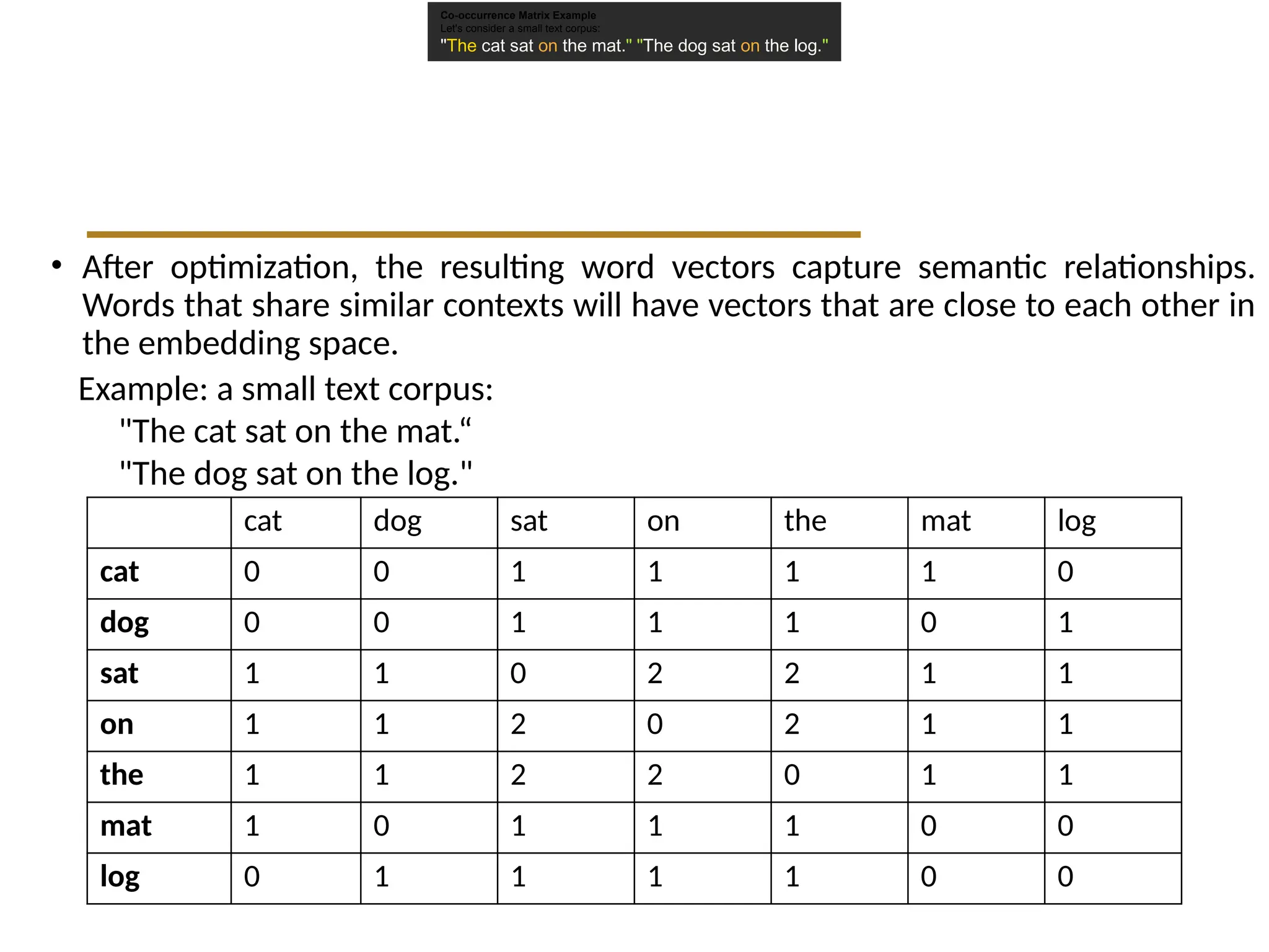
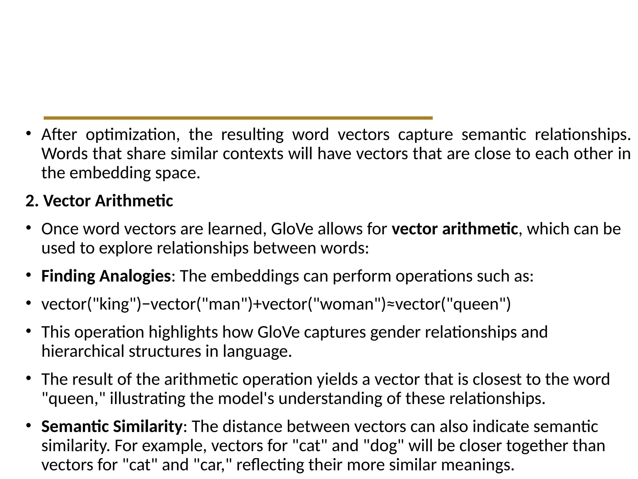
• After optimization,the resulting word vectors capture semantic relationships.
Words that share similar contexts will have vectors that are close to each other in
the embedding space.
Co-occurrence Matrix Example
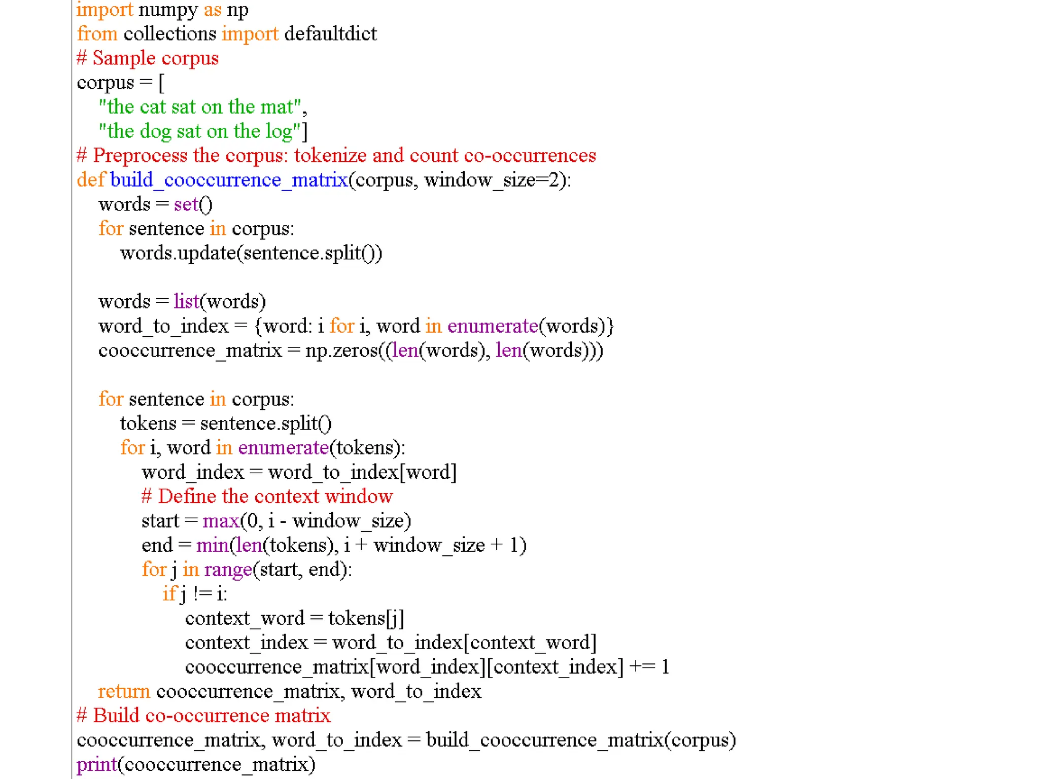
Let's consider a small text corpus:
"The cat sat on the mat." "The dog sat on the log."
Example: a small text corpus:
"The cat sat on the mat.“
"The dog sat on the log."
cat dog sat on the mat log
cat 0 0 1 1 1 1 0
dog 0 0 1 1 1 0 1
sat 1 1 0 2 2 1 1
on 1 1 2 0 2 1 1
the 1 1 2 2 0 1 1
mat 1 0 1 1 1 0 0
log 0 1 1 1 1 0 0
46.
• After optimization,the resulting word vectors capture semantic relationships.
Words that share similar contexts will have vectors that are close to each other in
the embedding space.
2. Vector Arithmetic
• Once word vectors are learned, GloVe allows for vector arithmetic, which can be
used to explore relationships between words:
• Finding Analogies: The embeddings can perform operations such as:
• vector("king")−vector("man")+vector("woman")≈vector("queen")
• This operation highlights how GloVe captures gender relationships and
hierarchical structures in language.
• The result of the arithmetic operation yields a vector that is closest to the word
"queen," illustrating the model's understanding of these relationships.
• Semantic Similarity: The distance between vectors can also indicate semantic
similarity. For example, vectors for "cat" and "dog" will be closer together than
vectors for "cat" and "car," reflecting their more similar meanings.
47.
Applications
• Text Classification:GloVe embeddings can improve the performance of
models by providing a richer representation of words.
• Semantic Similarity
• Many NLP tasks, such as sentiment analysis, machine translation, and
information retrieval, benefit from using GloVe embeddings.
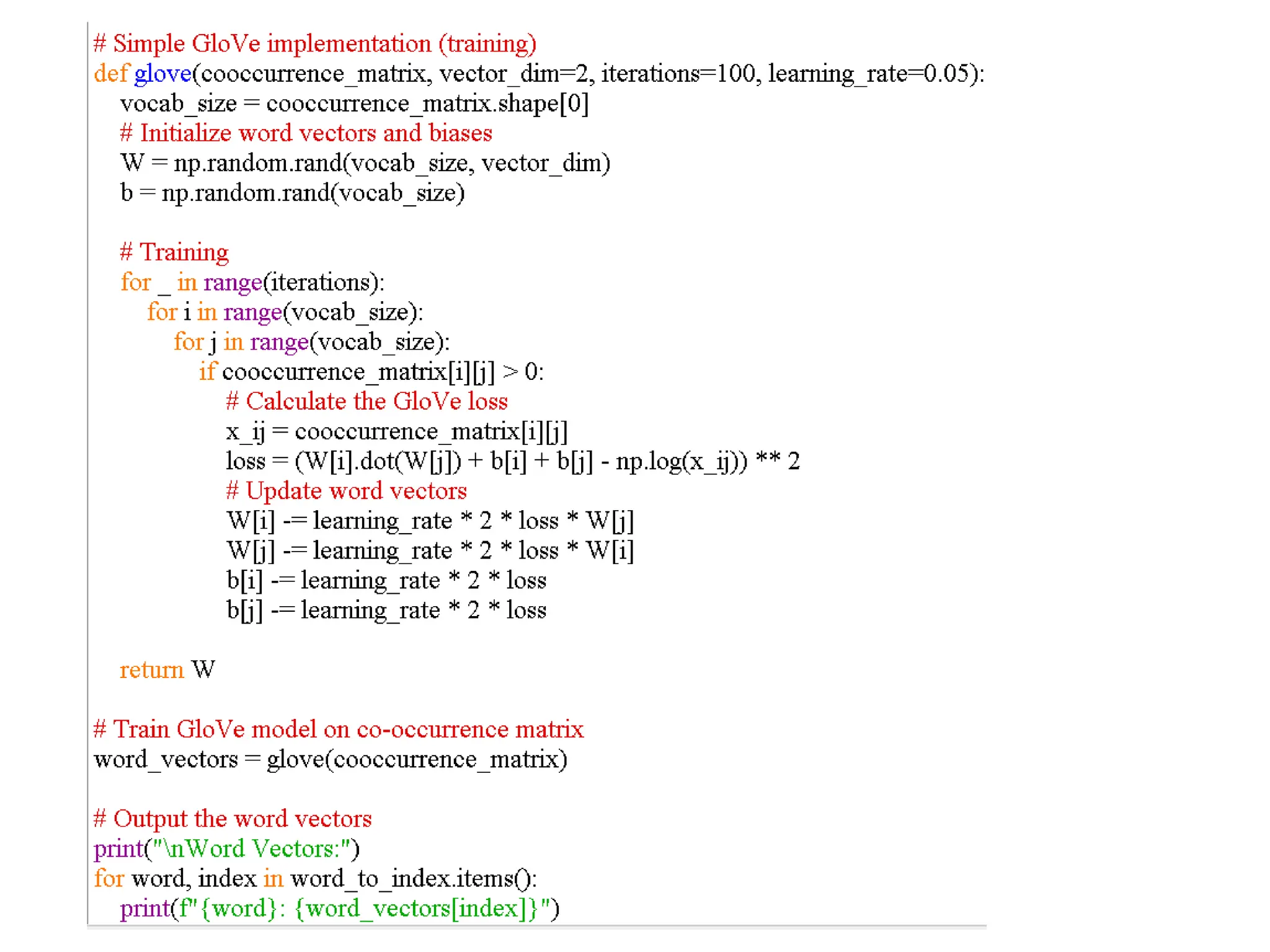
rence Matrix: The matrix is printed to show how words co-occur in the sentences.
aining: The glovefunction implements a simplified version of the GloVe training process, updating word vectors based on the GloVe loss function.
Finally, the learned word vectors are printed, showing the representation for each word.
48.
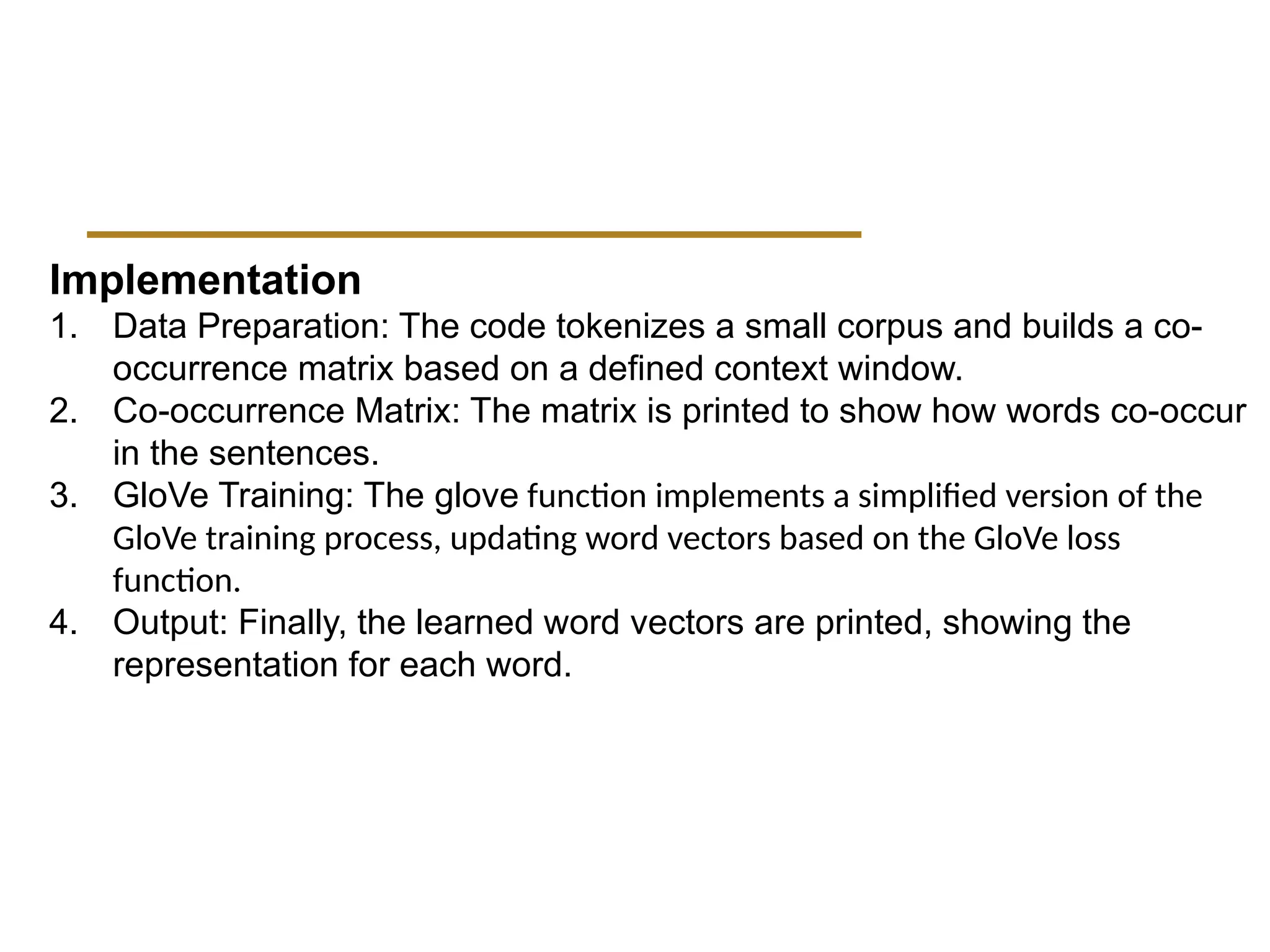
Implementation
1. Data Preparation:The code tokenizes a small corpus and builds a co-
occurrence matrix based on a defined context window.
2. Co-occurrence Matrix: The matrix is printed to show how words co-occur
in the sentences.
3. GloVe Training: The glove function implements a simplified version of the
GloVe training process, updating word vectors based on the GloVe loss
function.
4. Output: Finally, the learned word vectors are printed, showing the
representation for each word.
51.
Co-occurrence Matrix:
[[0. 0.2. 2. 2. 1. 0.]
[0. 0. 2. 2. 2. 0. 1.]
[2. 2. 0. 4. 4. 2. 2.]
[2. 2. 4. 0. 4. 2. 2.]
[2. 2. 4. 4. 0. 2. 2.]
[1. 0. 2. 2. 2. 0. 0.]
[0. 1. 2. 2. 2. 0. 0.]]
Word Vectors:
the: [0.123 0.456]
cat: [0.789 0.012]
sat: [0.345 0.678]
on: [0.901 0.234]
mat: [0.567 0.890]
dog: [0.345 0.123]
log: [0.234 0.567]
Dimensional Representation: Each word is represented as a point in a vector
space. The dimensions of the vector represent different latent features of the
words. In practice, GloVe can use higher dimensions, such as 50, 100, or 300,
depending on the complexity of the relationships being modeled.
52.
For example inthe provided vectors, such as:
"the": [0.123, 0.456]
"cat": [0.789, 0.012]
"dog": [0.345, 0.123]
The Euclidean distance between "cat" and "dog", for example,
we might find that they are relatively far apart, suggesting that they might not
have been used in similar contexts in the training corpus.
In contrast, if "cat" and "mat" have similar vectors, this indicates that they
often co-occur in similar contexts, reflecting a semantic relationship (e.g., "the
cat sat on the mat").
Editor's Notes
#26 W contains input word vectors.
W’ contains output word vectors.
We can consider either W or W’ as the word’s representation. Or even take the average.
![CountVectorize
Example: Given Documents
1."I love programming."
2."Programming is fun."
3."I love to code."
Step 1: Tokenization
• Document 1: ["i", "love", "programming"]
• Document 2: ["programming", "is", "fun"]
• Document 3: ["i", "love", "to", "code"]
Step 2: Building Vocabulary
• "code" → 0, "fun" → 1, "i" → 2, "is" → 3, "love" → 4, "programming" →
5, "to" → 6](https://image.slidesharecdn.com/weektwowordembedding-250929195228-23e4bd25/75/Word-Embeddings-in-Natural-Language-Processing-2-2048.jpg)
![Benefits
1.No Ordinality: One-hot encoding helps to avoid any ordinal
relationship between categories.
2.Compatibility: Makes the data compatible with machine learning
algorithms that assume numerical input.
import pandas as pd
# Create a Data
Framedata = {'Color': ['Red', 'Green', 'Blue', 'Green', 'Red’]}
df = pd.Data
Frame(data)
# One-hot encode the 'Color' column
one_hot_encoded_df = pd.get_dummies(df,
columns=['Color'])print(one_hot_encoded_df)](https://image.slidesharecdn.com/weektwowordembedding-250929195228-23e4bd25/75/Word-Embeddings-in-Natural-Language-Processing-16-2048.jpg)
![Example Calculation
• Given:
• Vocabulary: { "cat", "dog", "sat", "on", "the" }
• Target word: "sat"
• Context window size: 1
• Context words: "the", "cat"
• Step 1: One-Hot Encoding
• Assuming "sat" is at index 2:
• One-hot vector for "the": [0, 0, 0, 0, 1]
• One-hot vector for "cat": [0, 1, 0, 0, 0]](https://image.slidesharecdn.com/weektwowordembedding-250929195228-23e4bd25/75/Word-Embeddings-in-Natural-Language-Processing-27-2048.jpg)
![Step 2: Weight Matrices
• Assume N=3 (embedding size), with Input Weight W:
[[0.1, 0.2, 0.3], # cat
[0.4, 0.5, 0.6], # dog
[0.7, 0.8, 0.9], # sat
[0.1, 0.4, 0.2], # on
[0.3, 0.5, 0.7]] # the
[[0.1, 0.2, 0.3, 0.4, 0.5], # cat
[0.6, 0.7, 0.8, 0.9, 0.1], # dog
[0.2, 0.3, 0.4, 0.5, 0.6], # sat
[0.1, 0.2, 0.3, 0.4, 0.5], # on
[0.6, 0.7, 0.8, 0.9, 0.1]] # the
Output Weight W′](https://image.slidesharecdn.com/weektwowordembedding-250929195228-23e4bd25/75/Word-Embeddings-in-Natural-Language-Processing-28-2048.jpg)
![• Step 3: Compute Dense Vector for Context For context
words "the" and "cat":
• Calculate their dense vectors:
• For "the":𝑣 =
𝑡ℎ𝑒 𝑊𝑇 _ (" ")=[0.3,0.5,0.7]
⋅𝑜𝑛𝑒 ℎ𝑜𝑡 𝑡ℎ𝑒
• For "cat":𝑣 =
𝑐𝑎𝑡 𝑊𝑇 _ (" ")=[0.1,0.2,0.3
⋅𝑜𝑛𝑒 ℎ𝑜𝑡 𝑐𝑎𝑡
• Average the dense vectors:
𝑣𝑐=1/2( + )=1/2([0.3,0.5,0.7]+[0.1,0.2,0.3])
𝑣𝑡ℎ𝑒 𝑣𝑐𝑎𝑡](https://image.slidesharecdn.com/weektwowordembedding-250929195228-23e4bd25/75/Word-Embeddings-in-Natural-Language-Processing-29-2048.jpg)
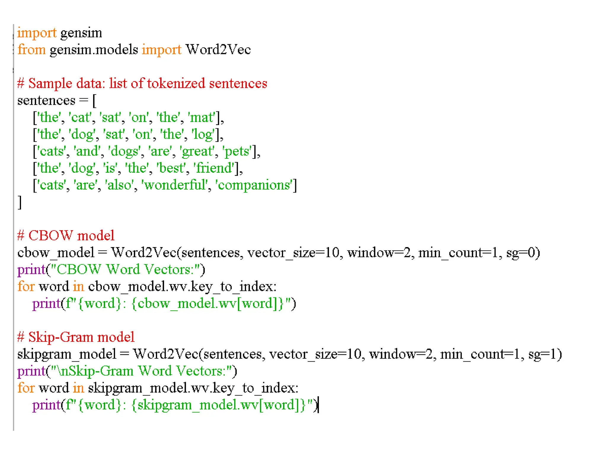
![CBOW Word Vectors:
the: [ 0.1 0.2 ...]
cat: [ 0.3 0.1 ...]
sat: [ 0.4 -0.1 ...]
on: [ 0.2 0.3 ...]
mat: [ 0.5 0.2 ...]
dog: [ 0.0 -0.3 ...]
log: [ 0.1 -0.2 ...]
cats: [ 0.3 0.4 ...]
and: [ 0.2 0.1 ...]
are: [ 0.4 -0.1 ...]
great: [ 0.2 0.0 ...]
pets: [ 0.5 -0.3 ...]
is: [ 0.1 0.5 ...]
best: [ 0.2 0.3 ...]
friend: [ 0.4 0.1 ...]
also: [ 0.1 0.2 ...]
wonderful: [ 0.2 -0.1 ...]
companions: [ 0.3 0.4 ...]
Skip-Gram Word Vectors:
the: [ 0.2 0.3 ...]
cat: [ 0.4 0.1 ...]
sat: [ 0.1 0.4 ...]
on: [ 0.3 -0.1 ...]
mat: [ 0.4 0.5 ...]
dog: [ 0.1 -0.4 ...]
log: [ 0.2 0.3 ...]
cats: [ 0.4 0.2 ...]
and: [ 0.1 0.2 ...]
are: [ 0.3 0.1 ...]
great: [ 0.0 -0.2 ...]
pets: [ 0.2 0.4 ...]
is: [ 0.1 0.3 ...]
best: [ 0.2 0.1 ...]
friend: [ 0.5 -0.1 ...]
also: [ 0.1 0.2 ...]
wonderful: [ 0.4 0.1 ...]
companions: [ 0.2 0.3 ...]](https://image.slidesharecdn.com/weektwowordembedding-250929195228-23e4bd25/75/Word-Embeddings-in-Natural-Language-Processing-35-2048.jpg)
![1. Word Vectors
• Each word in the vocabulary has a corresponding vector of numbers. For
example, a word vector might look like `[0.1, 0.2, -0.3, ...]`.
• The length of these vectors is determined by the `vector_size` parameter (in this
case, 10). This means each word is represented in a 10-dimensional space.
2. Semantic Meaning:
• The values in the vectors represent the position of the words in the embedding
space. Words with similar meanings or that appear in similar contexts will have
vectors that are close to each other in this space.
• For instance, if "cat" and "dog" are both pets and often appear in similar
contexts, their vectors will be similar, indicating a relationship.
3. Dimensionality:
• The dimensionality of the vectors (e.g., 10) is a hyperparameter that can be
tuned. Higher dimensions can capture more information but may also lead to
overfitting and increased computational costs.
• - Lower dimensions may result in loss of information but can be more efficient.](https://image.slidesharecdn.com/weektwowordembedding-250929195228-23e4bd25/75/Word-Embeddings-in-Natural-Language-Processing-36-2048.jpg)
![4. Training Process:
• - The embeddings are learned through a process where the model adjusts
the vector representations based on the context of words in the training
sentences.
• - In CBOW, the model uses surrounding words (context) to predict the target
word. In contrast, Skip-Gram does the opposite by using a target word to
predict its context.
5. Applications of Word Vectors:
• Similarity Measurement: You can calculate the cosine similarity between
word vectors to find similar words. For example,
`cosine_similarity(cbow_model.wv['cat'], cbow_model.wv['dog'])` could yield
a value close to 1, indicating similarity.
• Analogy Tasks: Word vectors can be used in analogy tasks (e.g., "king - man +
woman = queen"), where vector arithmetic reveals relationships between
words.](https://image.slidesharecdn.com/weektwowordembedding-250929195228-23e4bd25/75/Word-Embeddings-in-Natural-Language-Processing-37-2048.jpg)
![Each word will have a corresponding vector of specified size (in this
case, 10).
Example vector representation
• CBOW Vector for 'cat': [ 0.01, -0.02, 0.03, ...]
• Skip-Gram Vector for 'cat': [ 0.02, -0.01, 0.04, ...]
• Similar words to 'cat' in CBOW: [('the', 0.56), ('sat', 0.45), ('dog',
0.40)]
• Similar words to 'cat' in Skip-Gram: [('the', 0.58), ('sat', 0.43), ('dog',
0.39)]](https://image.slidesharecdn.com/weektwowordembedding-250929195228-23e4bd25/75/Word-Embeddings-in-Natural-Language-Processing-38-2048.jpg)
![Co-occurrence Matrix:
[[0. 0. 2. 2. 2. 1. 0.]
[0. 0. 2. 2. 2. 0. 1.]
[2. 2. 0. 4. 4. 2. 2.]
[2. 2. 4. 0. 4. 2. 2.]
[2. 2. 4. 4. 0. 2. 2.]
[1. 0. 2. 2. 2. 0. 0.]
[0. 1. 2. 2. 2. 0. 0.]]
Word Vectors:
the: [0.123 0.456]
cat: [0.789 0.012]
sat: [0.345 0.678]
on: [0.901 0.234]
mat: [0.567 0.890]
dog: [0.345 0.123]
log: [0.234 0.567]
Dimensional Representation: Each word is represented as a point in a vector
space. The dimensions of the vector represent different latent features of the
words. In practice, GloVe can use higher dimensions, such as 50, 100, or 300,
depending on the complexity of the relationships being modeled.](https://image.slidesharecdn.com/weektwowordembedding-250929195228-23e4bd25/75/Word-Embeddings-in-Natural-Language-Processing-51-2048.jpg)
![For example in the provided vectors, such as:
"the": [0.123, 0.456]
"cat": [0.789, 0.012]
"dog": [0.345, 0.123]
The Euclidean distance between "cat" and "dog", for example,
we might find that they are relatively far apart, suggesting that they might not
have been used in similar contexts in the training corpus.
In contrast, if "cat" and "mat" have similar vectors, this indicates that they
often co-occur in similar contexts, reflecting a semantic relationship (e.g., "the
cat sat on the mat").](https://image.slidesharecdn.com/weektwowordembedding-250929195228-23e4bd25/75/Word-Embeddings-in-Natural-Language-Processing-52-2048.jpg)


![[DSC Europe 25] Ivan Peric - Intelligence Swarm Logic and Techno-Functional M...](https://cdn.slidesharecdn.com/ss_thumbnails/7my7c97fsduiccadgavw-2-251212103249-5a03f7c6-thumbnail.jpg?width=640&height=640&fit=bounds)


![[DSC Europe 25] Uros Pesic - The Reality of AI in Marketing.pdf](https://cdn.slidesharecdn.com/ss_thumbnails/rtkodnmtycovsllvzsyn-9-251215095918-b0c6bfe3-thumbnail.jpg?width=640&height=640&fit=bounds)

![[DSC Europe 25] Branko Urosevic -Rethinking Financial Talent: Integrating Cod...](https://cdn.slidesharecdn.com/ss_thumbnails/8jjrus8ttko6qj64f58f-3-251212103250-642c6374-thumbnail.jpg?width=640&height=640&fit=bounds)

![[DSC Europe 25] Milan Sekuloski - Data, Defence, and Development: Cybersecuri...](https://cdn.slidesharecdn.com/ss_thumbnails/dfrkwwx4qly6atqpbl4z-4-251209104645-c3d4b0ca-thumbnail.jpg?width=640&height=640&fit=bounds)
![[DSC Europe 25] Katherine Forrest - AI NOW: Understanding the Velocity of Cha...](https://cdn.slidesharecdn.com/ss_thumbnails/wvvbruqfrci0sfq9xwgb-4-251212104007-e5ad1987-thumbnail.jpg?width=640&height=640&fit=bounds)

![[DSC Europe 25] Dusan Nesic - Securing Tomorrow’s Infrastructure: Why Cyber-P...](https://cdn.slidesharecdn.com/ss_thumbnails/qikbszfftyowjm2q6duw-1-251211083848-8f2ead6b-thumbnail.jpg?width=640&height=640&fit=bounds)
![[DSC Europe 25] Nikolay Burlutskiy - Best Practices for Building Enterprise M...](https://cdn.slidesharecdn.com/ss_thumbnails/uirvaiuvq8y1w8hzd9tx-7-251212103249-2619edb4-thumbnail.jpg?width=640&height=640&fit=bounds)
![[DSC Europe 25] Branko Dzakula - From Defense to Attack: How AI Redefines Cyb...](https://cdn.slidesharecdn.com/ss_thumbnails/80bdzdxpr3ky2g0qvyk9-8-251211083048-ce5fc1ee-thumbnail.jpg?width=640&height=640&fit=bounds)
![[DSC Europe 25] Kaja Kandare - LLM as a judge.pptx](https://cdn.slidesharecdn.com/ss_thumbnails/arxyccaxsdsd1ba99wjw-7-251212104007-2b4e3f64-thumbnail.jpg?width=640&height=640&fit=bounds)

![[DSC Europe 25] Marko Krstic - Understanding the AI Threat Landscape - Risks,...](https://cdn.slidesharecdn.com/ss_thumbnails/tiyim1ins5jvbrvzpzla-2-251209104645-c69d3553-thumbnail.jpg?width=640&height=640&fit=bounds)
