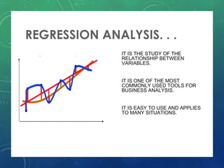
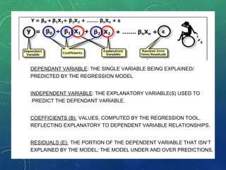
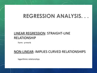
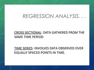
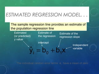
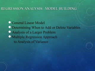
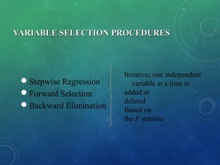
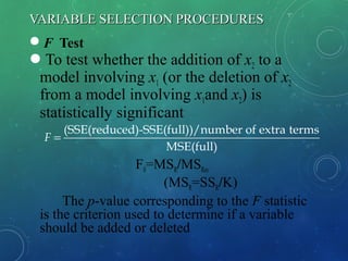
WELCOME TO OUR PRESENTATION
PRESENTED BY:
Md . Sohag
Em@il : sohag.0315@gmail.com
Daffodil international University
INTRODUCTION. . .
• FATHER OF REGRESSION ANALYSIS
CARL F. GAUSS (1777-1855).
• CONTRIBUTIONS TO PHYSICS, MATHEMATICS &
ASTRONOMY.
• THE TERM “REGRESSION” WAS FIRST USED IN
1877 BY FRANCIS GALTON.
REGRESSION ANALYSIS. . .
• IT IS THE STUDY OF THE
RELATIONSHIP BETWEEN
VARIABLES.
• IT IS ONE OF THE MOST
COMMONLY USED TOOLS FOR
BUSINESS ANALYSIS.
• IT IS EASY TO USE AND APPLIES
TO MANY SITUATIONS.
REGRESSION TYPES. . .
• SIMPLE REGRESSION: SINGLE
EXPLANATORY VARIABLE
• MULTIPLE REGRESSION: INCLUDES ANY
NUMBER OF EXPLANATORY VARIABLES.
• DEPENDANT VARIABLE: THE SINGLE VARIABLE BEING EXPLAINED/
• PREDICTED BY THE REGRESSION MODEL
• INDEPENDENT VARIABLE: THE EXPLANATORY VARIABLE(S) USED TO
• PREDICT THE DEPENDANT VARIABLE.
• COEFFICIENTS (Β): VALUES, COMPUTED BY THE REGRESSION TOOL,
• REFLECTING EXPLANATORY TO DEPENDENT VARIABLE RELATIONSHIPS.
• RESIDUALS (Ε): THE PORTION OF THE DEPENDENT VARIABLE THAT ISN’T
• EXPLAINED BY THE MODEL; THE MODEL UNDER AND OVER PREDICTIONS.
REGRESSION ANALYSIS. . .
• LINEAR REGRESSION: STRAIGHT-LINE
RELATIONSHIP
– Form: y=mx+b
• NON-LINEAR: IMPLIES CURVED RELATIONSHIPS
–
logarithmic relationships
REGRESSION ANALYSIS. . .
• CROSS SECTIONAL: DATA GATHERED FROM THE
SAME TIME PERIOD
• TIME SERIES: INVOLVES DATA OBSERVED OVER
EQUALLY SPACED POINTS IN TIME.
SIMPLE LINEAR REGRESSION MODEL. . .
TYPES OF REGRESSION MODELS. . .
xbbyˆ 10i +=
The sample regression line provides an estimate of
the population regression line
ESTIMATED REGRESSION MODEL. . .
Estimate of
the regression
intercept
Estimate of the
regression slope
Estimated
(or predicted)
y value
Independent
variable
The individual random error terms ei have a mean of zero
REGRESSION ANALYSIS: MODEL BUILDINGREGRESSION ANALYSIS: MODEL BUILDING
General Linear Model
Determining When to Add or Delete Variables
Analysis of a Larger Problem
Multiple Regression Approach
to Analysis of Variance
GENERAL LINEAR MODELGENERAL LINEAR MODEL
Modelsin which theparameters(β0, β1, . . . , βp) all haveexponentsof onearecalled
linear models.
 First-Order Model with OnePredictor Variable
y x= + +β β ε0 1 1y x= + +β β ε0 1 1
VARIABLE SELECTION PROCEDURESVARIABLE SELECTION PROCEDURES
Stepwise Regression
Forward Selection
Backward Elimination
Iterative; one independent
variable at a time is
added or
deleted
Based on
the F statistic
VARIABLE SELECTION PROCEDURESVARIABLE SELECTION PROCEDURES
F Test
To test whether the addition of x2 to a
model involving x1 (or the deletion of x2
from a model involving x1and x2) is
statistically significant
F0=MSR/MSRes
(MSR=SSR/K)
The p-value corresponding to the F statistic
is the criterion used to determine if a variable
should be added or deleted
(SSE(reduced)-SSE(full))/number of extra terms
MSE(full)
F =
FORWARD SELECTIONFORWARD SELECTION
This procedure is similar to stepwise-regression,
but does not permit a variable to be deleted.
This forward-selection procedure starts with no
independent variables.
It adds variables one at a time as long as a
significant reduction in the error sum of squares
(SSE) can be achieved.
BACKWARD ELIMINATIONBACKWARD ELIMINATION
This procedure begins with a model that includes all the
independent variables the modeler wants considered.
It then attempts to delete one variable at a time by
determining whether the least significant variable currently
in the model can be removed because its p-value is less than
the user-specified or default value.
Once a variable has been removed from the model it cannot
re enter at a subsequent step.
Example1-:From the following data obtain the two regression equations
using the method of Least Squares.
X 3 2 7 4 8
Y 6 1 8 5 9
Solution-:
X Y XY X2
Y2
3 6 18 9 36
2 1 2 4 1
7 8 56 49 64
4 5 20 16 25
8 9 72 64 81
∑ = 24X ∑ = 29Y ∑ =168XY 1422
=∑ X 2072
=∑Y
Example2-: from the previous data obtain the regression equations by
Taking deviations from the actual means of X and Y series.
X 3 2 7 4 8
Y 6 1 8 5 9
X Y x2
y2
xy
3 6 -1.8 0.2 3.24 0.04 -0.36
2 1 -2.8 -4.8 7.84 23.04 13.44
7 8 2.2 2.2 4.84 4.84 4.84
4 5 -0.8 -0.8 0.64 0.64 0.64
8 9 3.2 3.2 10.24 10.24 10.24
XXx −= YYy −=
∑ = 24X ∑ = 29Y 8.26
2
=∑x 8.28=∑ xy8.382
=∑ y∑ = 0x 0∑ =y
Solution-:
Example-: From the data given in previous example calculate regression
equations by assuming 7 as the mean of X series and 6 as the mean of Y series.
X Y
Dev. From
assu.
Mean 7
(dx)=X-7
Dev. From
assu. Mean
6 (dy)=Y-6 dxdy
3 6 -4 16 0 0 0
2 1 -5 25 -5 25 +25
7 8 0 0 2 4 0
4 5 -3 9 -1 1 +3
8 9 1 1 3 9 +3
Solution-:
2
xd 2
yd
∑ = 24X ∑ = 29Y ∑ −= 11xd ∑ −= 1yd∑ = 512
xd ∑ = 392
yd ∑ = 31yxdd

Regression analysis

  • 1.
    WELCOME TO OURPRESENTATION PRESENTED BY: Md . Sohag Em@il : sohag.0315@gmail.com Daffodil international University
  • 3.
    INTRODUCTION. . . •FATHER OF REGRESSION ANALYSIS CARL F. GAUSS (1777-1855). • CONTRIBUTIONS TO PHYSICS, MATHEMATICS & ASTRONOMY. • THE TERM “REGRESSION” WAS FIRST USED IN 1877 BY FRANCIS GALTON.
  • 4.
    REGRESSION ANALYSIS. .. • IT IS THE STUDY OF THE RELATIONSHIP BETWEEN VARIABLES. • IT IS ONE OF THE MOST COMMONLY USED TOOLS FOR BUSINESS ANALYSIS. • IT IS EASY TO USE AND APPLIES TO MANY SITUATIONS.
  • 5.
    REGRESSION TYPES. .. • SIMPLE REGRESSION: SINGLE EXPLANATORY VARIABLE • MULTIPLE REGRESSION: INCLUDES ANY NUMBER OF EXPLANATORY VARIABLES.
  • 6.
    • DEPENDANT VARIABLE:THE SINGLE VARIABLE BEING EXPLAINED/ • PREDICTED BY THE REGRESSION MODEL • INDEPENDENT VARIABLE: THE EXPLANATORY VARIABLE(S) USED TO • PREDICT THE DEPENDANT VARIABLE. • COEFFICIENTS (Β): VALUES, COMPUTED BY THE REGRESSION TOOL, • REFLECTING EXPLANATORY TO DEPENDENT VARIABLE RELATIONSHIPS. • RESIDUALS (Ε): THE PORTION OF THE DEPENDENT VARIABLE THAT ISN’T • EXPLAINED BY THE MODEL; THE MODEL UNDER AND OVER PREDICTIONS.
  • 7.
    REGRESSION ANALYSIS. .. • LINEAR REGRESSION: STRAIGHT-LINE RELATIONSHIP – Form: y=mx+b • NON-LINEAR: IMPLIES CURVED RELATIONSHIPS – logarithmic relationships
  • 8.
    REGRESSION ANALYSIS. .. • CROSS SECTIONAL: DATA GATHERED FROM THE SAME TIME PERIOD • TIME SERIES: INVOLVES DATA OBSERVED OVER EQUALLY SPACED POINTS IN TIME.
  • 9.
  • 10.
  • 11.
    xbbyˆ 10i += Thesample regression line provides an estimate of the population regression line ESTIMATED REGRESSION MODEL. . . Estimate of the regression intercept Estimate of the regression slope Estimated (or predicted) y value Independent variable The individual random error terms ei have a mean of zero
  • 12.
    REGRESSION ANALYSIS: MODELBUILDINGREGRESSION ANALYSIS: MODEL BUILDING General Linear Model Determining When to Add or Delete Variables Analysis of a Larger Problem Multiple Regression Approach to Analysis of Variance
  • 13.
    GENERAL LINEAR MODELGENERALLINEAR MODEL Modelsin which theparameters(β0, β1, . . . , βp) all haveexponentsof onearecalled linear models.  First-Order Model with OnePredictor Variable y x= + +β β ε0 1 1y x= + +β β ε0 1 1
  • 14.
    VARIABLE SELECTION PROCEDURESVARIABLESELECTION PROCEDURES Stepwise Regression Forward Selection Backward Elimination Iterative; one independent variable at a time is added or deleted Based on the F statistic
  • 15.
    VARIABLE SELECTION PROCEDURESVARIABLESELECTION PROCEDURES F Test To test whether the addition of x2 to a model involving x1 (or the deletion of x2 from a model involving x1and x2) is statistically significant F0=MSR/MSRes (MSR=SSR/K) The p-value corresponding to the F statistic is the criterion used to determine if a variable should be added or deleted (SSE(reduced)-SSE(full))/number of extra terms MSE(full) F =
  • 16.
    FORWARD SELECTIONFORWARD SELECTION Thisprocedure is similar to stepwise-regression, but does not permit a variable to be deleted. This forward-selection procedure starts with no independent variables. It adds variables one at a time as long as a significant reduction in the error sum of squares (SSE) can be achieved.
  • 17.
    BACKWARD ELIMINATIONBACKWARD ELIMINATION Thisprocedure begins with a model that includes all the independent variables the modeler wants considered. It then attempts to delete one variable at a time by determining whether the least significant variable currently in the model can be removed because its p-value is less than the user-specified or default value. Once a variable has been removed from the model it cannot re enter at a subsequent step.
  • 18.
    Example1-:From the followingdata obtain the two regression equations using the method of Least Squares. X 3 2 7 4 8 Y 6 1 8 5 9 Solution-: X Y XY X2 Y2 3 6 18 9 36 2 1 2 4 1 7 8 56 49 64 4 5 20 16 25 8 9 72 64 81 ∑ = 24X ∑ = 29Y ∑ =168XY 1422 =∑ X 2072 =∑Y
  • 19.
    Example2-: from theprevious data obtain the regression equations by Taking deviations from the actual means of X and Y series. X 3 2 7 4 8 Y 6 1 8 5 9 X Y x2 y2 xy 3 6 -1.8 0.2 3.24 0.04 -0.36 2 1 -2.8 -4.8 7.84 23.04 13.44 7 8 2.2 2.2 4.84 4.84 4.84 4 5 -0.8 -0.8 0.64 0.64 0.64 8 9 3.2 3.2 10.24 10.24 10.24 XXx −= YYy −= ∑ = 24X ∑ = 29Y 8.26 2 =∑x 8.28=∑ xy8.382 =∑ y∑ = 0x 0∑ =y Solution-:
  • 20.
    Example-: From thedata given in previous example calculate regression equations by assuming 7 as the mean of X series and 6 as the mean of Y series. X Y Dev. From assu. Mean 7 (dx)=X-7 Dev. From assu. Mean 6 (dy)=Y-6 dxdy 3 6 -4 16 0 0 0 2 1 -5 25 -5 25 +25 7 8 0 0 2 4 0 4 5 -3 9 -1 1 +3 8 9 1 1 3 9 +3 Solution-: 2 xd 2 yd ∑ = 24X ∑ = 29Y ∑ −= 11xd ∑ −= 1yd∑ = 512 xd ∑ = 392 yd ∑ = 31yxdd