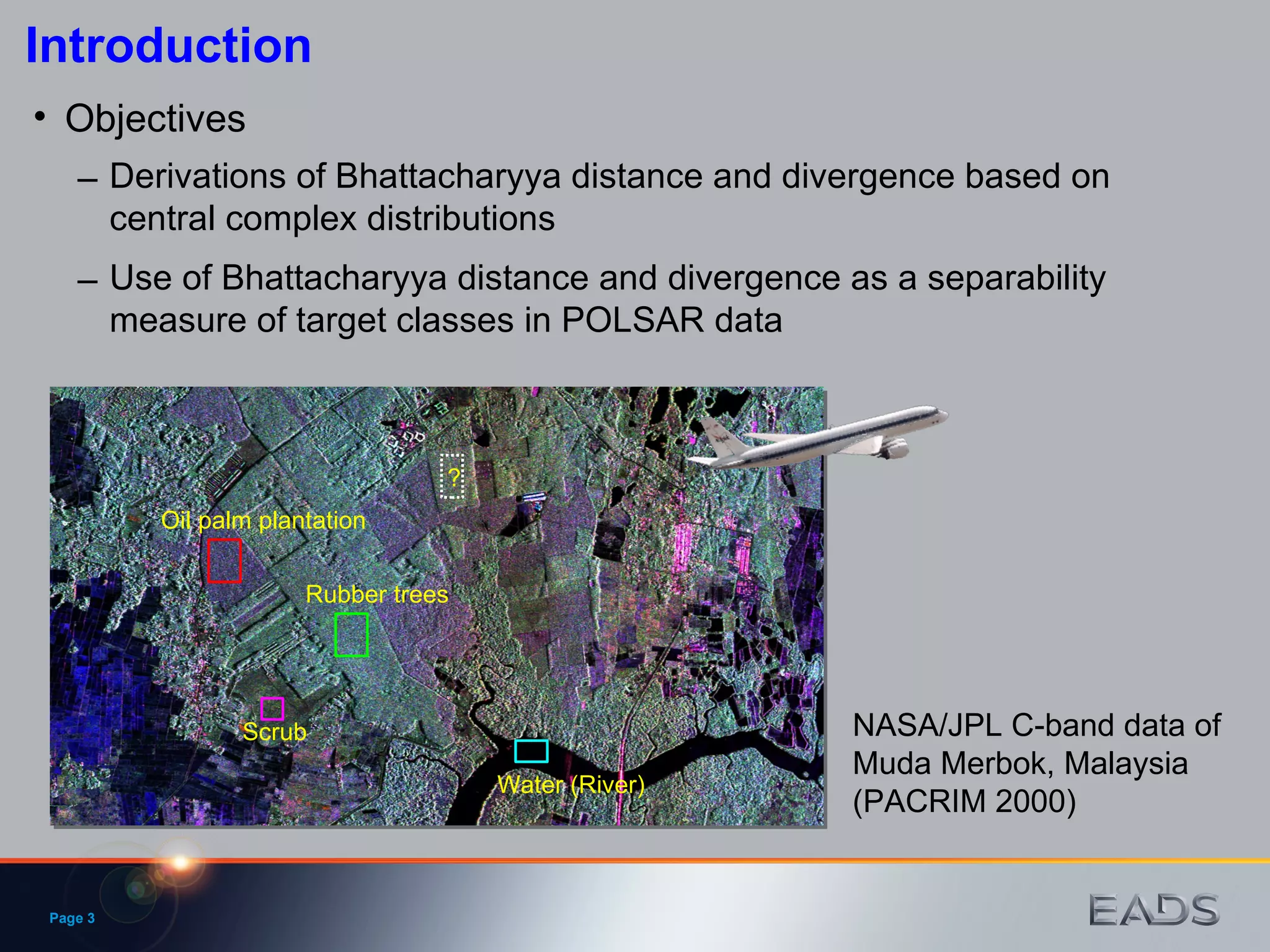
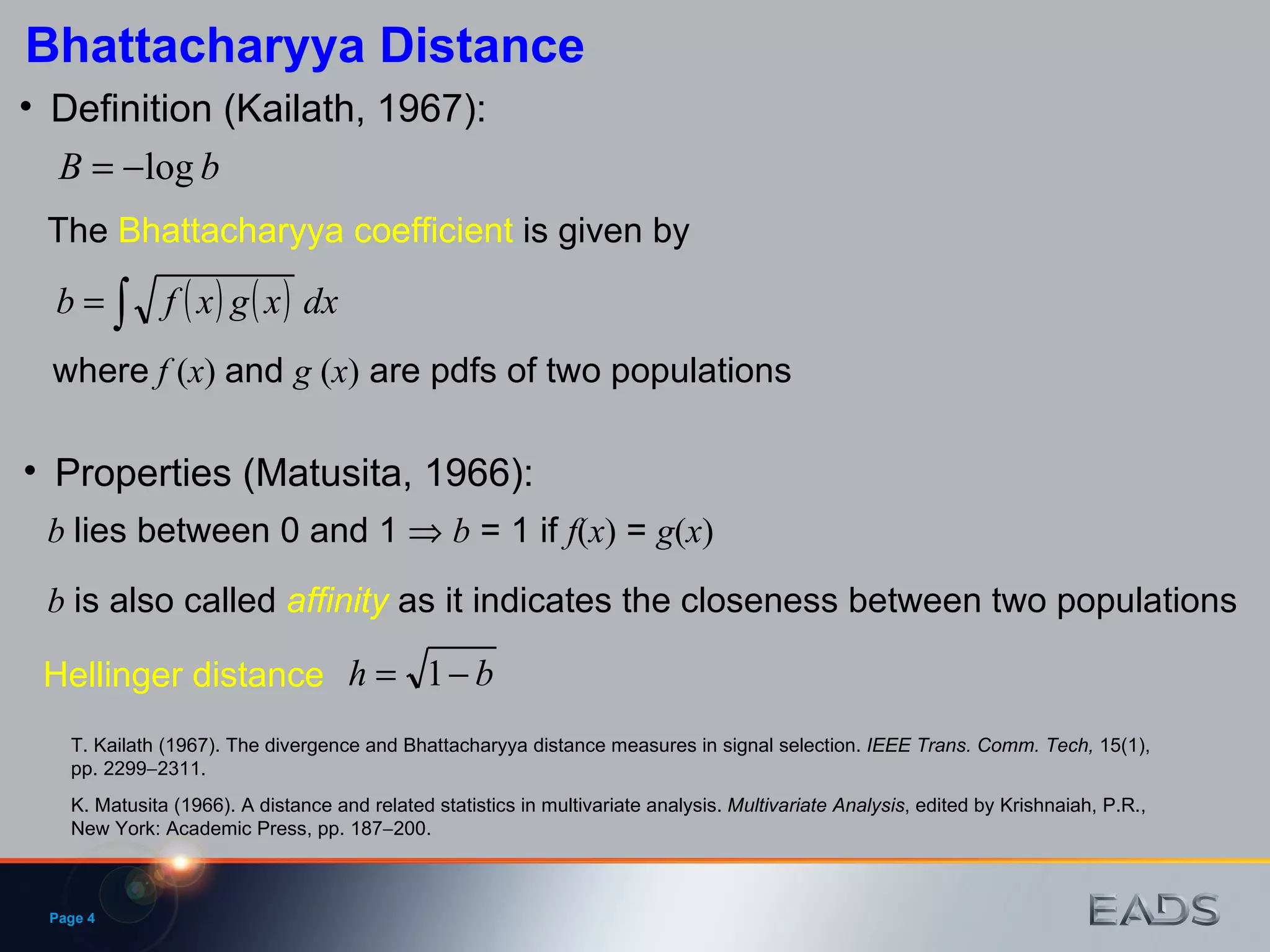
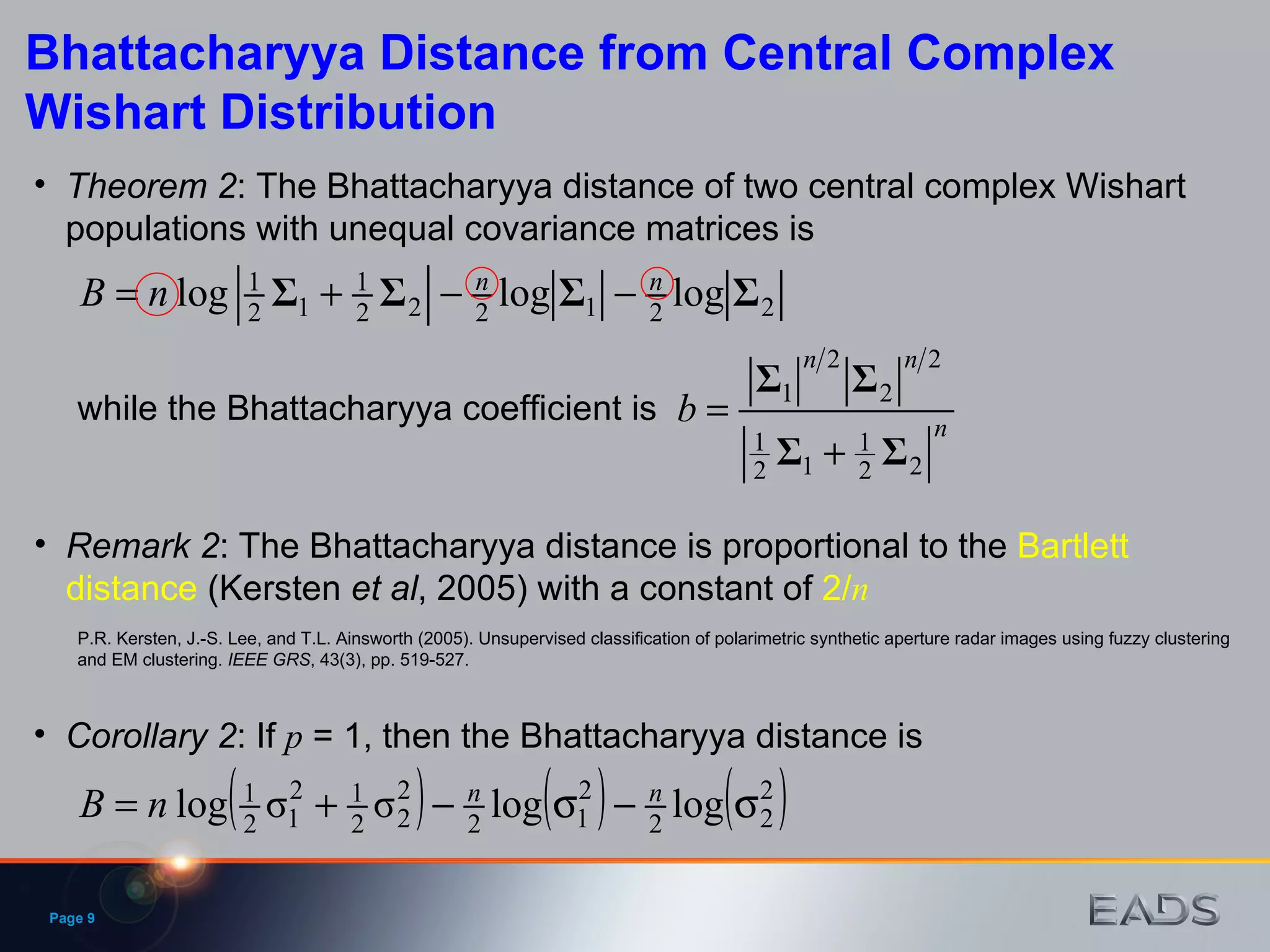
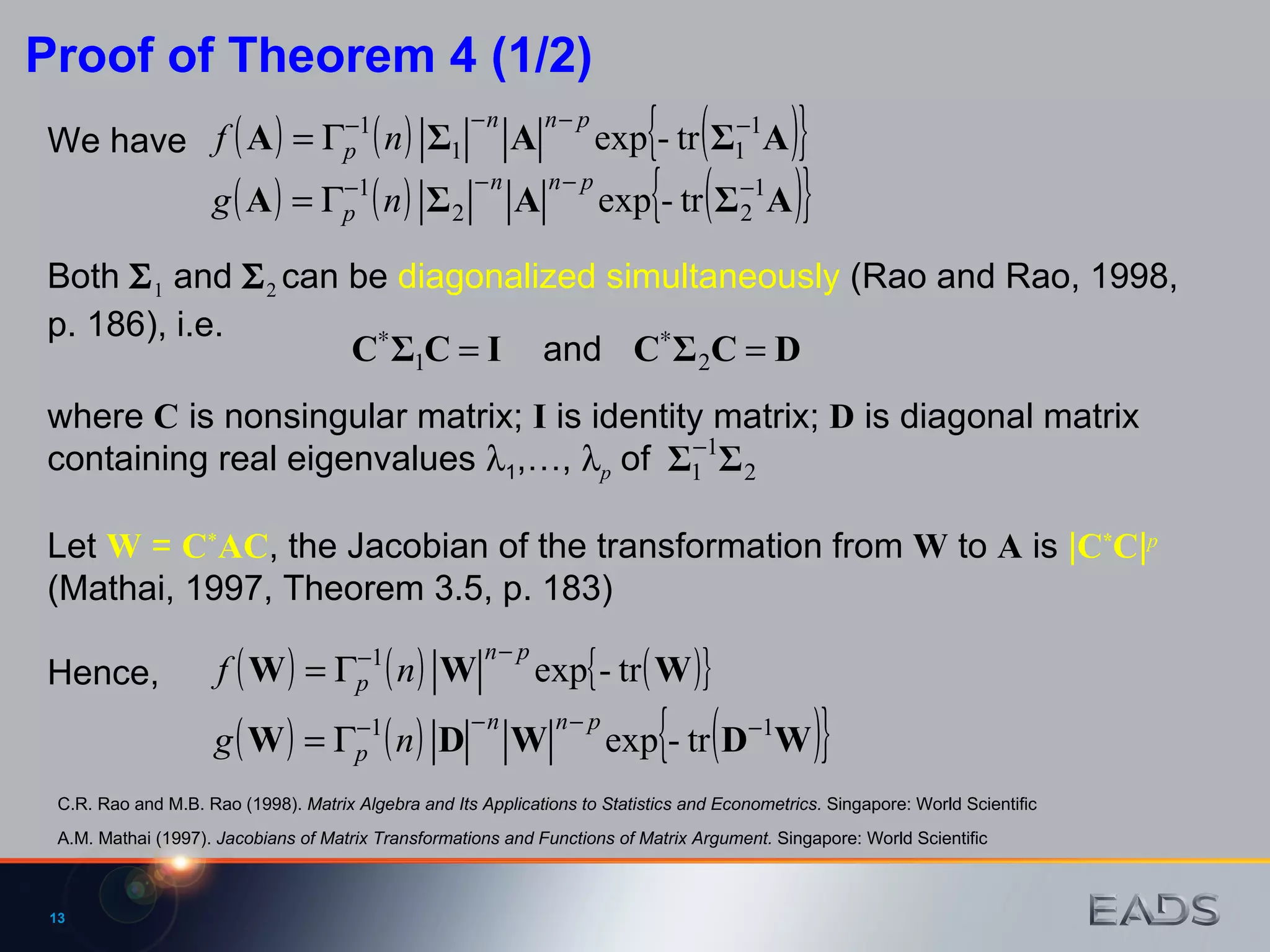
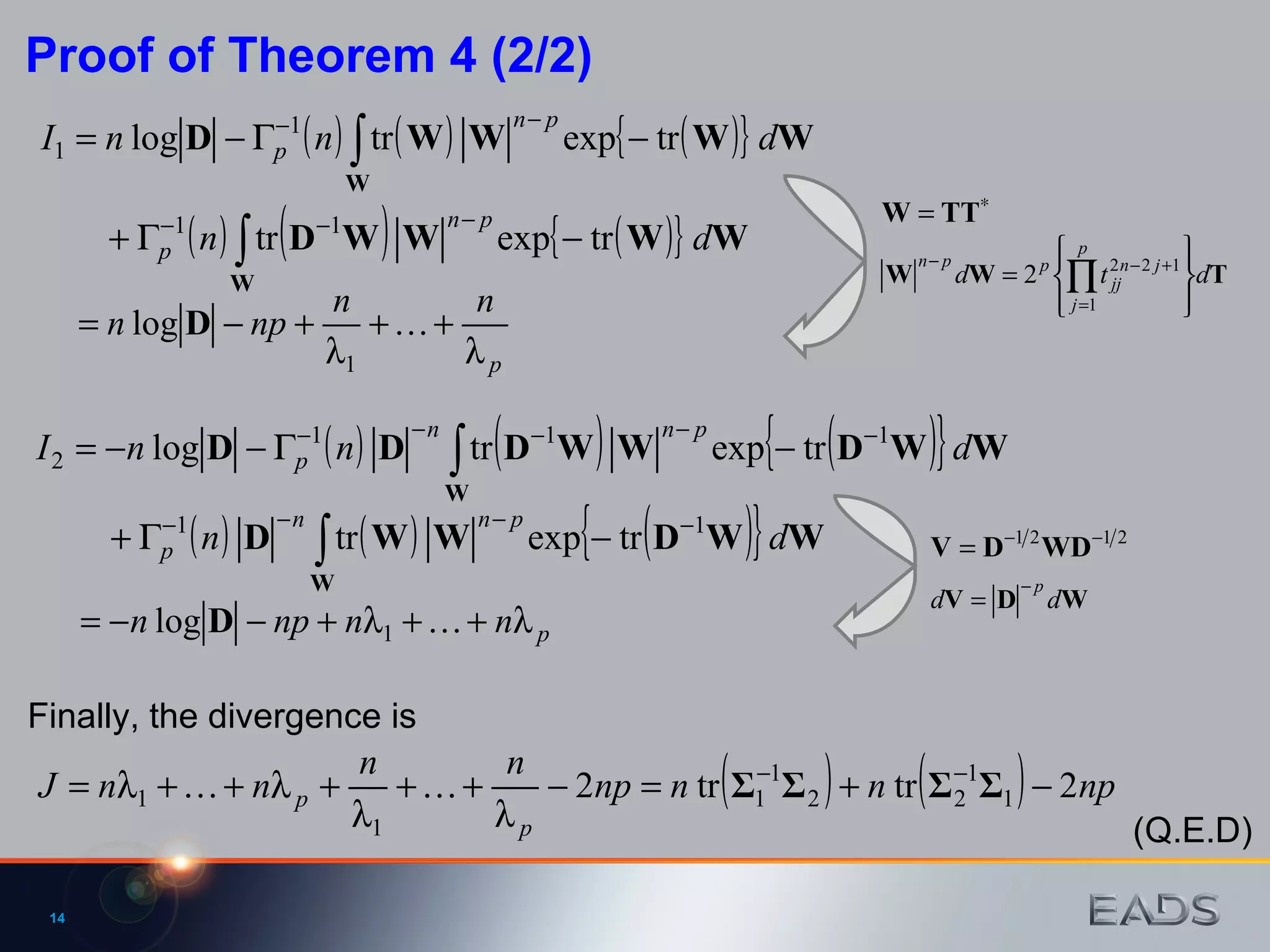
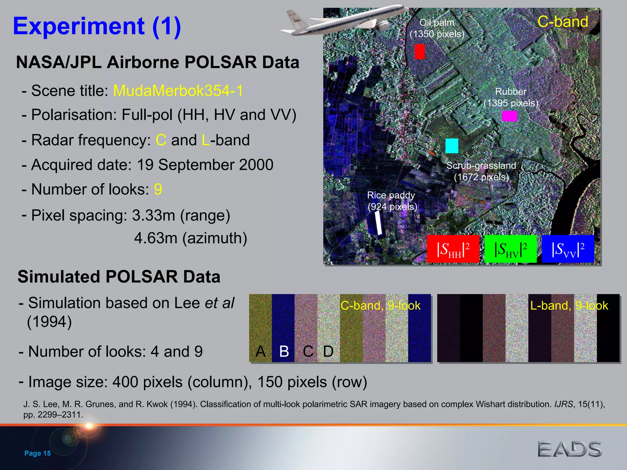
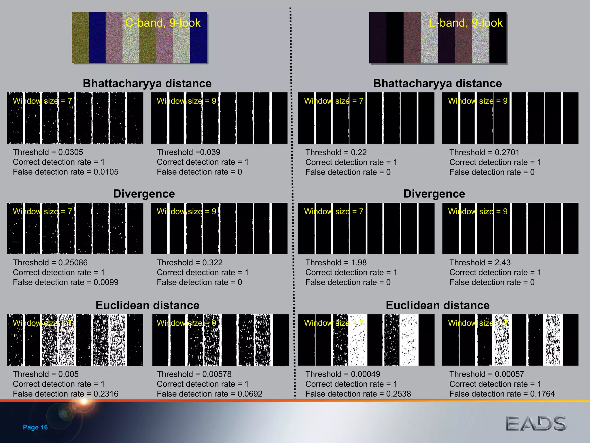
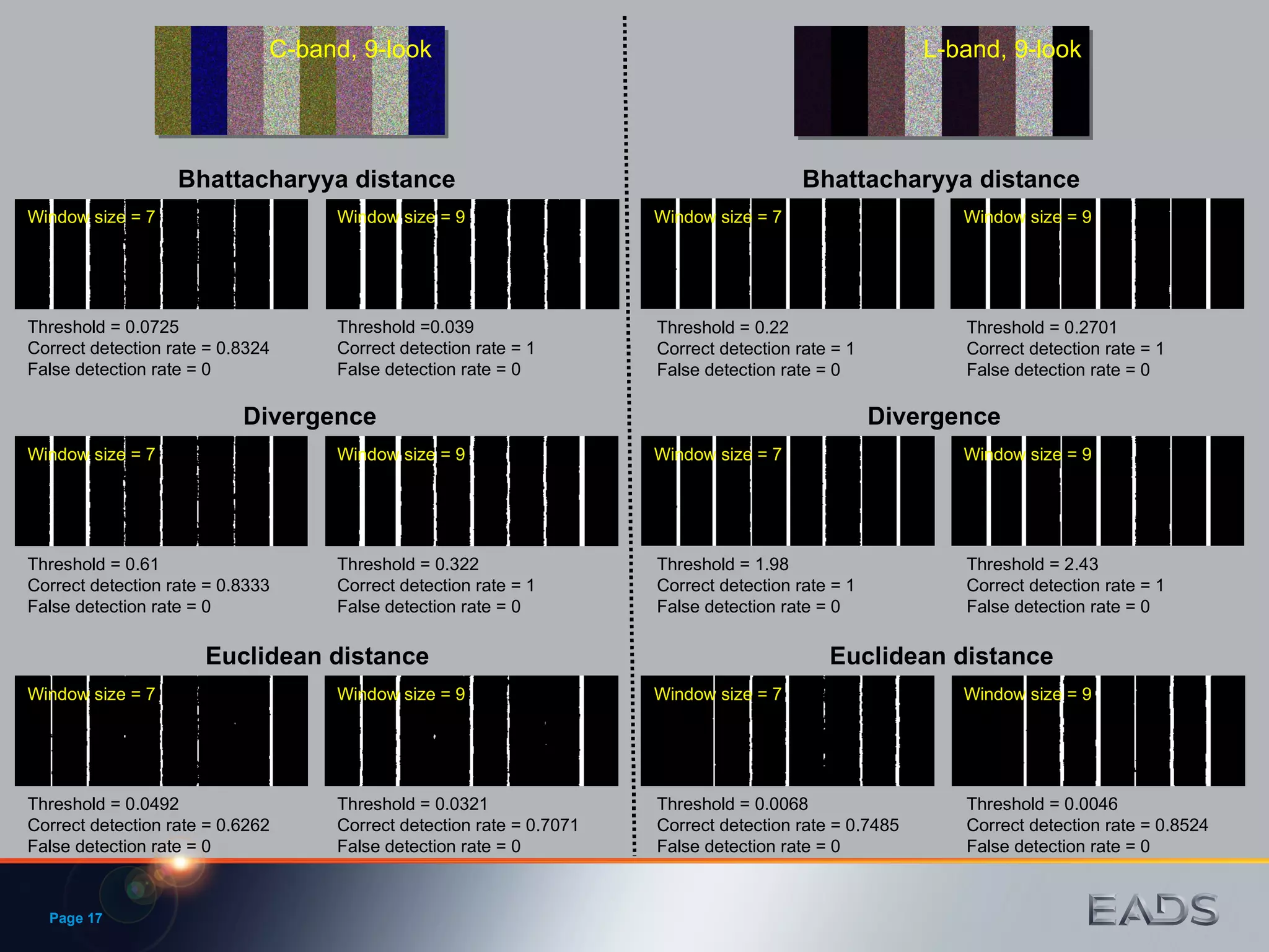
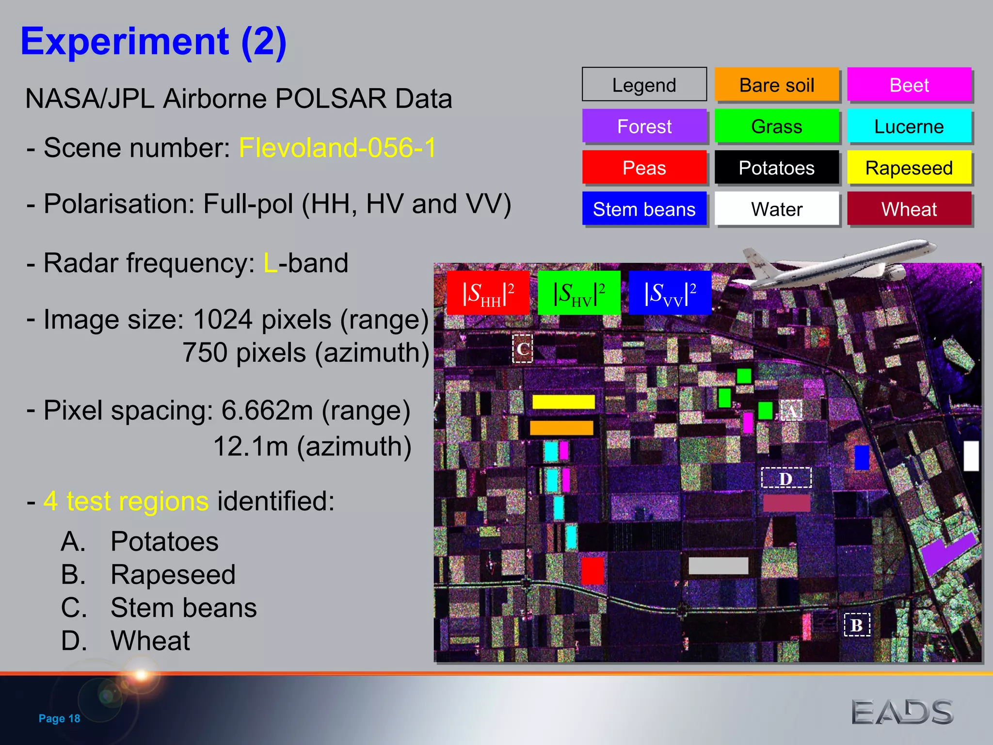
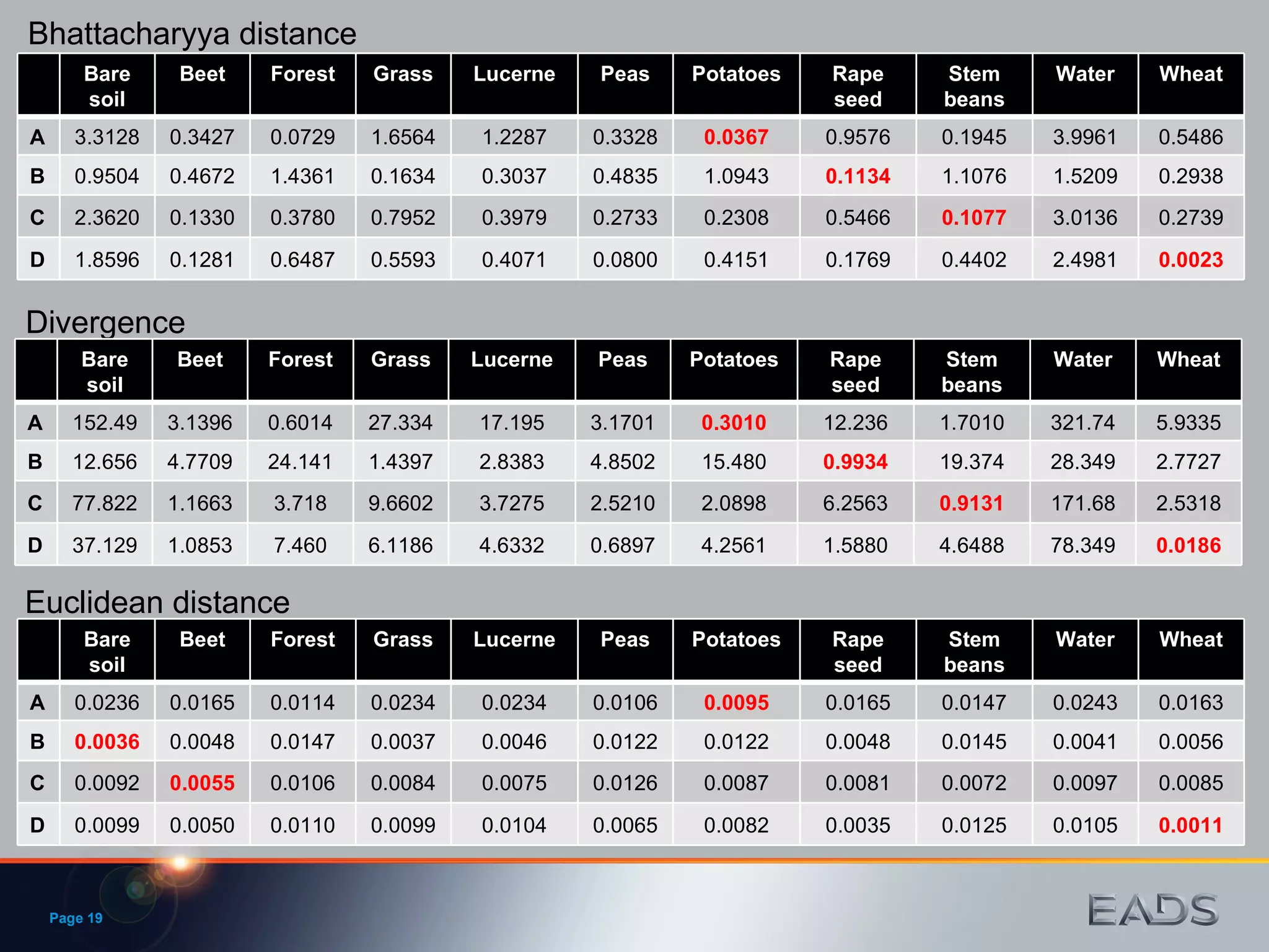
Derivation of Separability Measures Based on Central Complex Gaussian and Wishart Distributions Ken Yoong LEE and Timo Rolf Bretschneider July 2011 EADS Innovation Works Singapore
Page  Content Overview Objectives Divergence Experiments Simulated POLSAR data NASA/JPL POLSAR data Based on central complex Gaussian distribution Based on central complex Wishart distribution Bhattacharyya distance  Summary Based on central complex Gaussian distribution Based on central complex Wishart distribution
Page  Introduction Objectives Rubber trees Oil palm plantation Water (River) Scrub ? NASA/JPL C-band data of Muda Merbok, Malaysia (PACRIM 2000) Use of Bhattacharyya distance and divergence as a separability measure of target classes in POLSAR data Derivations of Bhattacharyya distance and divergence based on central complex distributions
Definition (Kailath, 1967): T. Kailath (1967). The divergence and Bhattacharyya distance measures in signal selection.  IEEE Trans. Comm. Tech,  15(1), pp. 2299  2311. The  Bhattacharyya coefficient  is given by where   f  ( x )  and  g  ( x )  are pdfs of two populations Properties (Matusita, 1966): K. Matusita (1966). A distance and related statistics in multivariate analysis.  Multivariate Analysis , edited by Krishnaiah, P.R., New York: Academic Press, pp. 187  200. b   lies between 0 and 1     b  = 1 if  f ( x )  =  g ( x )   b   is also called  affinity  as it indicates the closeness between two populations Bhattacharyya Distance Page  Hellinger distance
Page  Scattering Vector and Central Complex Gaussian Distribution Scattering vector  z  can be assumed to follow  p -dimensional central complex Gaussian distribution (Kong  et   al , 1987): J. A. Kong, A. A. Swartz, H. A. Yueh, L. M. Novak, and R. T. Shin (1987). Identification of terrain cover using the optimum polarimetric classifier.  JEWA , 2(2) pp. 171  194. Scattering vector  z  in single-look single-frequency polarimetric synthetic aperture radar data:
Page  Bhattacharyya Distance from Central Complex Gaussian Distribution Theorem 1 : The Bhattacharyya distance of two central complex multivariate Gaussian populations with unequal covariance matrices is Corollary 1 : If  p  = 1, then the Bhattacharyya distance is while the Bhattacharyya coefficient is Remark 1 : The application of Bhattacharyya distance for contrast analysis can be found in Morio  et   al  (2008) J. Morio, P. Réfrégier, F. Goudail, P.C. Dubois-Fernandez, and X. Dupuis (2008). Information theory-based approach for contrast analysis in polarimetric and/or interferometric SAR images.  IEEE Trans. GRS , 46, pp. 2185  2196
Use of the following integration rules: and Hence, the Bhattacharyya coefficient is  while the Bhattacharyya distance is  (Q.E.D) Now, the Bhattacharyya coefficient is Proof of Theorem 1
Page  Covariance Matrix and Complex Wishart Distribution Hermitian matrix  A  =  n   C  can be assumed to follow central complex Wishart distribution (Lee  et   al , 1994): J. S. Lee, M. R. Grunes, and R. Kwok (1994). Classification of multi-look polarimetric SAR imagery based on complex Wishart distribution.  IJRS , 15(11), pp. 2299  2311. Covariance matrix  C  in  n -look single-frequency polarimetric synthetic aperture radar data:
Page  Bhattacharyya Distance from Central Complex Wishart Distribution Theorem 2 : The Bhattacharyya distance of two central complex Wishart populations with unequal covariance matrices is Corollary 2 : If  p  = 1, then the Bhattacharyya distance is while the Bhattacharyya coefficient is Remark 2 : The Bhattacharyya distance is proportional to the  Bartlett distance  (Kersten  et   al , 2005) with a constant of  2/ n P.R. Kersten, J.-S. Lee, and T.L. Ainsworth (2005). Unsupervised classification of polarimetric synthetic aperture radar images using fuzzy clustering and EM clustering.  IEEE GRS , 43(3), pp. 519-527.
The Jacobian of  B  to  A :  is  Complex multivariate gamma function Hence, the Bhattacharyya coefficient is  (Q.E.D) Now, the Bhattacharyya coefficient is Proof of Theorem 2 A.M. Mathai (1997).  Jacobians of Matrix Transformations and Functions of Matrix Argument.  Singapore: World Scientific (Mathai, 1997, Th. 3.5, p. 183)
Definition (Jeffreys, 1946; Kullback, 1959): H. Jeffreys (1946). An invariant form for the prior probability in estimation problems.  Proc. Royal Soc. London  ( Ser. A ) ,  186(1007), pp. 453  461. where the functions   f ( x )  and  g ( x )  are pdf of two populations Properties: S. Kullback (1959).  Information Theory and Statistics , New York: John Wiley. J   is zero if if  f ( x )  =  g ( x ) , which implies no divergence between a distribution and itself Divergence Page  and I 1  or  I 2  is also known as Kullback-Leibler divergence
Page  Divergence Theorem 3 : The divergence of two  p -dimensional central complex Gaussian populations with unequal covariance matrices is Theorem 4 : The divergence of two  p -dimensional central complex Wishart populations with unequal covariance matrices is Remark 3 : The divergence is proportional to the  symmetrized normalized log-likelihood distance  (Anfinsen  et   al , 2007) with a constant of  (2 n ) -1 S.N. Anfinsen, R. Jensen, and T. Eltolf (2007). Spectral clustering of polarimetric SAR data with Wishart-derived distance measures.  Proc. POLinSAR 2007,  Available at earth.esa.int/workshops/polinsar2007/papers/140_anfinsen.pdf
Both   1  and   2  can be  diagonalized simultaneously  (Rao and Rao, 1998, p. 186), i.e.  and We have Proof of Theorem 4 (1/2) where  C  is nonsingular matrix;  I  is identity matrix;  D  is diagonal matrix containing real eigenvalues   1 ,…,   p  of  Let  W  =  C * AC , the Jacobian of the transformation from  W  to  A  is  | C * C | p   (Mathai, 1997, Theorem 3.5, p. 183)  Hence, A.M. Mathai (1997).  Jacobians of Matrix Transformations and Functions of Matrix Argument.  Singapore: World Scientific C.R. Rao and M.B. Rao (1998).  Matrix Algebra and Its Applications to Statistics and Econometrics.  Singapore: World Scientific
Proof of Theorem 4 (2/2) Finally, the divergence is (Q.E.D)
Page  Experiment (1) Scrub-grassland (1672 pixels) Oil palm (1350 pixels) Rubber (1395 pixels) Rice paddy  (924 pixels) NASA/JPL Airborne POLSAR Data - Radar frequency:  C  and  L -band - Polarisation: Full-pol (HH, HV and VV) Pixel spacing: 3.33m (range) 4.63m (azimuth) - Scene title:  MudaMerbok354-1 | S HH | 2 | S HV | 2 | S VV | 2 C-band Image size: 400 pixels (column), 150 pixels (row) Simulated POLSAR Data - Number of looks:  9 A  B   C  D  C-band, 9-look L-band, 9-look - Number of looks: 4 and 9 J. S. Lee, M. R. Grunes, and R. Kwok (1994). Classification of multi-look polarimetric SAR imagery based on complex Wishart distribution.  IJRS , 15(11), pp. 2299  2311. - Simulation based on Lee  et   al  (1994) - Acquired date: 19 September 2000
Page  Bhattacharyya distance Window size = 7 Divergence Euclidean distance C-band, 9-look L-band, 9-look Window size = 9 Window size = 7 Window size = 9 Window size = 7 Window size = 9 Window size = 7 Window size = 9 Window size = 7 Window size = 9 Window size = 7 Window size = 9 Threshold =0.039  Correct detection rate = 1 False detection rate = 0 Threshold = 0.0305 Correct detection rate = 1 False detection rate = 0.0105 Threshold = 0.322 Correct detection rate = 1 False detection rate = 0 Threshold = 0.25086 Correct detection rate = 1 False detection rate = 0.0099 Threshold = 0.00578 Correct detection rate = 1 False detection rate = 0.0692 Threshold = 0.005 Correct detection rate = 1 False detection rate = 0.2316 Threshold = 0.2701 Correct detection rate = 1 False detection rate = 0 Threshold = 0.22 Correct detection rate = 1 False detection rate = 0 Threshold = 2.43 Correct detection rate = 1 False detection rate = 0 Threshold = 1.98 Correct detection rate = 1 False detection rate = 0 Threshold = 0.00057 Correct detection rate = 1 False detection rate = 0.1764 Threshold = 0.00049 Correct detection rate = 1 False detection rate = 0.2538 Bhattacharyya distance Divergence Euclidean distance
Page  Bhattacharyya distance Window size = 7 Divergence Euclidean distance C-band, 9-look L-band, 9-look Window size = 9 Window size = 7 Window size = 9 Window size = 7 Window size = 9 Window size = 7 Window size = 9 Window size = 7 Window size = 9 Window size = 7 Window size = 9 Threshold =0.039  Correct detection rate = 1 False detection rate = 0 Threshold = 0.0725 Correct detection rate = 0.8324 False detection rate = 0 Threshold = 0.322 Correct detection rate = 1 False detection rate = 0 Threshold = 0.61 Correct detection rate = 0.8333 False detection rate = 0 Threshold = 0.0321 Correct detection rate = 0.7071 False detection rate = 0 Threshold = 0.0492 Correct detection rate = 0.6262 False detection rate = 0 Threshold = 0.2701 Correct detection rate = 1 False detection rate = 0 Threshold = 0.22 Correct detection rate = 1 False detection rate = 0 Threshold = 2.43 Correct detection rate = 1 False detection rate = 0 Threshold = 1.98 Correct detection rate = 1 False detection rate = 0 Threshold = 0.0046  Correct detection rate = 0.8524 False detection rate = 0 Threshold = 0.0068 Correct detection rate = 0.7485 False detection rate = 0 Bhattacharyya distance Divergence Euclidean distance
Page  NASA/JPL Airborne POLSAR Data - Radar frequency:  L -band - Polarisation: Full-pol (HH, HV and VV) Pixel spacing: 6.662m (range) 12.1m (azimuth) - Scene number:  Flevoland-056-1 Bare soil Beet Forest Grass Lucerne Potatoes Stem beans Water Wheat Peas Rapeseed Legend | S HH | 2 | S HV | 2 | S VV | 2 Image size: 1024 pixels (range) 750 pixels (azimuth) Experiment (2) Potatoes Rapeseed Stem beans Wheat -  4 test regions  identified:
Page  Bhattacharyya distance Divergence Euclidean distance Bare soil Beet Forest Grass Lucerne Peas Potatoes Rape seed Stem beans Water Wheat A 3.3128 0.3427 0.0729 1.6564 1.2287 0.3328 0.0367 0.9576 0.1945 3.9961 0.5486 B 0.9504 0.4672 1.4361 0.1634 0.3037 0.4835 1.0943 0.1134 1.1076 1.5209 0.2938 C 2.3620 0.1330 0.3780 0.7952 0.3979 0.2733 0.2308 0.5466 0.1077 3.0136 0.2739 D 1.8596 0.1281 0.6487 0.5593 0.4071 0.0800 0.4151 0.1769 0.4402 2.4981 0.0023 Bare soil Beet Forest Grass Lucerne Peas Potatoes Rape seed Stem beans Water Wheat A 152.49 3.1396 0.6014 27.334 17.195 3.1701 0.3010 12.236 1.7010 321.74 5.9335 B 12.656 4.7709 24.141 1.4397 2.8383 4.8502 15.480 0.9934 19.374 28.349 2.7727 C 77.822 1.1663 3.718 9.6602 3.7275 2.5210 2.0898 6.2563 0.9131 171.68 2.5318 D 37.129 1.0853 7.460 6.1186 4.6332 0.6897 4.2561 1.5880 4.6488 78.349 0.0186 Bare soil Beet Forest Grass Lucerne Peas Potatoes Rape seed Stem beans Water Wheat A 0.0236 0.0165 0.0114 0.0234 0.0234 0.0106 0.0095 0.0165 0.0147 0.0243 0.0163 B 0.0036 0.0048 0.0147 0.0037 0.0046 0.0122 0.0122 0.0048 0.0145 0.0041 0.0056 C 0.0092 0.0055 0.0106 0.0084 0.0075 0.0126 0.0087 0.0081 0.0072 0.0097 0.0085 D 0.0099 0.0050 0.0110 0.0099 0.0104 0.0065 0.0082 0.0035 0.0125 0.0105 0.0011
Page  Summary The Bhattacharyya distances for complex Gaussian and Wishart distributions differ only in term of the  number of degrees of freedom  ( number of looks  in POLSAR data) Same observation for the divergence The Bhattacharyya distance is proportional to the  Bartlett distance The divergence is proportional to the  symmetrized normalized log-likelihood distance Both the Bhattacharyya distance and the divergence perform consistently in measuring the separability of target classes The latter is more  computationally expensive  than the former
Colour palette EADS Innovation Works Singapore, Real-time Embedded Systems, IW-SI-I Page  28 July 2011
Page  Divergence Corollary 4 : If  p  = 1, then the divergence is Corollary 3 : If  p  = 1, then the divergence is
Both   1  and   2  can be diagonalized simultaneously (Rao and Rao, 1998, p. 186), i.e.  and We have Proof of Theorem 3 (1/2) where  C  is nonsingular matrix;  I  is identity matrix;  D  is diagonal matrix containing real eigenvalues   1 ,…,   p  of  and Let  w  =  C * z , the Jacobian of the transformation from  w  to  z  is | C * C |  (Mathai, 1997)  Hence, and A.M. Mathai (1997).  Jacobians of Matrix Transformations and Functions of Matrix Argument.  Singapore: World Scientific C.R. Rao and M.B. Rao (1998).  Matrix Algebra and Its Applications to Statistics and Econometrics.  Singapore: World Scientific
Proof of Theorem 3 (2/2) Finally, the divergence is (Q.E.D)
Page  Edge Templates 7  7 9  9 Euclidean Distance where b ij  is the matrix element of   2 a ij  is the matrix element of   1

DERIVATION OF SEPARABILITY MEASURES BASED ON CENTRAL COMPLEX GAUSSIAN AND WISHART DISTRIBUTIONS

  • 1.
    Derivation of SeparabilityMeasures Based on Central Complex Gaussian and Wishart Distributions Ken Yoong LEE and Timo Rolf Bretschneider July 2011 EADS Innovation Works Singapore
  • 2.
    Page ContentOverview Objectives Divergence Experiments Simulated POLSAR data NASA/JPL POLSAR data Based on central complex Gaussian distribution Based on central complex Wishart distribution Bhattacharyya distance Summary Based on central complex Gaussian distribution Based on central complex Wishart distribution
  • 3.
    Page IntroductionObjectives Rubber trees Oil palm plantation Water (River) Scrub ? NASA/JPL C-band data of Muda Merbok, Malaysia (PACRIM 2000) Use of Bhattacharyya distance and divergence as a separability measure of target classes in POLSAR data Derivations of Bhattacharyya distance and divergence based on central complex distributions
  • 4.
    Definition (Kailath, 1967):T. Kailath (1967). The divergence and Bhattacharyya distance measures in signal selection. IEEE Trans. Comm. Tech, 15(1), pp. 2299  2311. The Bhattacharyya coefficient is given by where f ( x ) and g ( x ) are pdfs of two populations Properties (Matusita, 1966): K. Matusita (1966). A distance and related statistics in multivariate analysis. Multivariate Analysis , edited by Krishnaiah, P.R., New York: Academic Press, pp. 187  200. b lies between 0 and 1  b = 1 if f ( x ) = g ( x ) b is also called affinity as it indicates the closeness between two populations Bhattacharyya Distance Page Hellinger distance
  • 5.
    Page ScatteringVector and Central Complex Gaussian Distribution Scattering vector z can be assumed to follow p -dimensional central complex Gaussian distribution (Kong et al , 1987): J. A. Kong, A. A. Swartz, H. A. Yueh, L. M. Novak, and R. T. Shin (1987). Identification of terrain cover using the optimum polarimetric classifier. JEWA , 2(2) pp. 171  194. Scattering vector z in single-look single-frequency polarimetric synthetic aperture radar data:
  • 6.
    Page BhattacharyyaDistance from Central Complex Gaussian Distribution Theorem 1 : The Bhattacharyya distance of two central complex multivariate Gaussian populations with unequal covariance matrices is Corollary 1 : If p = 1, then the Bhattacharyya distance is while the Bhattacharyya coefficient is Remark 1 : The application of Bhattacharyya distance for contrast analysis can be found in Morio et al (2008) J. Morio, P. Réfrégier, F. Goudail, P.C. Dubois-Fernandez, and X. Dupuis (2008). Information theory-based approach for contrast analysis in polarimetric and/or interferometric SAR images. IEEE Trans. GRS , 46, pp. 2185  2196
  • 7.
    Use of thefollowing integration rules: and Hence, the Bhattacharyya coefficient is while the Bhattacharyya distance is (Q.E.D) Now, the Bhattacharyya coefficient is Proof of Theorem 1
  • 8.
    Page CovarianceMatrix and Complex Wishart Distribution Hermitian matrix A = n C can be assumed to follow central complex Wishart distribution (Lee et al , 1994): J. S. Lee, M. R. Grunes, and R. Kwok (1994). Classification of multi-look polarimetric SAR imagery based on complex Wishart distribution. IJRS , 15(11), pp. 2299  2311. Covariance matrix C in n -look single-frequency polarimetric synthetic aperture radar data:
  • 9.
    Page BhattacharyyaDistance from Central Complex Wishart Distribution Theorem 2 : The Bhattacharyya distance of two central complex Wishart populations with unequal covariance matrices is Corollary 2 : If p = 1, then the Bhattacharyya distance is while the Bhattacharyya coefficient is Remark 2 : The Bhattacharyya distance is proportional to the Bartlett distance (Kersten et al , 2005) with a constant of 2/ n P.R. Kersten, J.-S. Lee, and T.L. Ainsworth (2005). Unsupervised classification of polarimetric synthetic aperture radar images using fuzzy clustering and EM clustering. IEEE GRS , 43(3), pp. 519-527.
  • 10.
    The Jacobian of B to A : is Complex multivariate gamma function Hence, the Bhattacharyya coefficient is (Q.E.D) Now, the Bhattacharyya coefficient is Proof of Theorem 2 A.M. Mathai (1997). Jacobians of Matrix Transformations and Functions of Matrix Argument. Singapore: World Scientific (Mathai, 1997, Th. 3.5, p. 183)
  • 11.
    Definition (Jeffreys, 1946;Kullback, 1959): H. Jeffreys (1946). An invariant form for the prior probability in estimation problems. Proc. Royal Soc. London ( Ser. A ) , 186(1007), pp. 453  461. where the functions f ( x ) and g ( x ) are pdf of two populations Properties: S. Kullback (1959). Information Theory and Statistics , New York: John Wiley. J is zero if if f ( x ) = g ( x ) , which implies no divergence between a distribution and itself Divergence Page and I 1 or I 2 is also known as Kullback-Leibler divergence
  • 12.
    Page DivergenceTheorem 3 : The divergence of two p -dimensional central complex Gaussian populations with unequal covariance matrices is Theorem 4 : The divergence of two p -dimensional central complex Wishart populations with unequal covariance matrices is Remark 3 : The divergence is proportional to the symmetrized normalized log-likelihood distance (Anfinsen et al , 2007) with a constant of (2 n ) -1 S.N. Anfinsen, R. Jensen, and T. Eltolf (2007). Spectral clustering of polarimetric SAR data with Wishart-derived distance measures. Proc. POLinSAR 2007, Available at earth.esa.int/workshops/polinsar2007/papers/140_anfinsen.pdf
  • 13.
    Both 1 and  2 can be diagonalized simultaneously (Rao and Rao, 1998, p. 186), i.e. and We have Proof of Theorem 4 (1/2) where C is nonsingular matrix; I is identity matrix; D is diagonal matrix containing real eigenvalues  1 ,…,  p of Let W = C * AC , the Jacobian of the transformation from W to A is | C * C | p (Mathai, 1997, Theorem 3.5, p. 183) Hence, A.M. Mathai (1997). Jacobians of Matrix Transformations and Functions of Matrix Argument. Singapore: World Scientific C.R. Rao and M.B. Rao (1998). Matrix Algebra and Its Applications to Statistics and Econometrics. Singapore: World Scientific
  • 14.
    Proof of Theorem4 (2/2) Finally, the divergence is (Q.E.D)
  • 15.
    Page Experiment(1) Scrub-grassland (1672 pixels) Oil palm (1350 pixels) Rubber (1395 pixels) Rice paddy (924 pixels) NASA/JPL Airborne POLSAR Data - Radar frequency: C and L -band - Polarisation: Full-pol (HH, HV and VV) Pixel spacing: 3.33m (range) 4.63m (azimuth) - Scene title: MudaMerbok354-1 | S HH | 2 | S HV | 2 | S VV | 2 C-band Image size: 400 pixels (column), 150 pixels (row) Simulated POLSAR Data - Number of looks: 9 A B C D C-band, 9-look L-band, 9-look - Number of looks: 4 and 9 J. S. Lee, M. R. Grunes, and R. Kwok (1994). Classification of multi-look polarimetric SAR imagery based on complex Wishart distribution. IJRS , 15(11), pp. 2299  2311. - Simulation based on Lee et al (1994) - Acquired date: 19 September 2000
  • 16.
    Page Bhattacharyyadistance Window size = 7 Divergence Euclidean distance C-band, 9-look L-band, 9-look Window size = 9 Window size = 7 Window size = 9 Window size = 7 Window size = 9 Window size = 7 Window size = 9 Window size = 7 Window size = 9 Window size = 7 Window size = 9 Threshold =0.039 Correct detection rate = 1 False detection rate = 0 Threshold = 0.0305 Correct detection rate = 1 False detection rate = 0.0105 Threshold = 0.322 Correct detection rate = 1 False detection rate = 0 Threshold = 0.25086 Correct detection rate = 1 False detection rate = 0.0099 Threshold = 0.00578 Correct detection rate = 1 False detection rate = 0.0692 Threshold = 0.005 Correct detection rate = 1 False detection rate = 0.2316 Threshold = 0.2701 Correct detection rate = 1 False detection rate = 0 Threshold = 0.22 Correct detection rate = 1 False detection rate = 0 Threshold = 2.43 Correct detection rate = 1 False detection rate = 0 Threshold = 1.98 Correct detection rate = 1 False detection rate = 0 Threshold = 0.00057 Correct detection rate = 1 False detection rate = 0.1764 Threshold = 0.00049 Correct detection rate = 1 False detection rate = 0.2538 Bhattacharyya distance Divergence Euclidean distance
  • 17.
    Page Bhattacharyyadistance Window size = 7 Divergence Euclidean distance C-band, 9-look L-band, 9-look Window size = 9 Window size = 7 Window size = 9 Window size = 7 Window size = 9 Window size = 7 Window size = 9 Window size = 7 Window size = 9 Window size = 7 Window size = 9 Threshold =0.039 Correct detection rate = 1 False detection rate = 0 Threshold = 0.0725 Correct detection rate = 0.8324 False detection rate = 0 Threshold = 0.322 Correct detection rate = 1 False detection rate = 0 Threshold = 0.61 Correct detection rate = 0.8333 False detection rate = 0 Threshold = 0.0321 Correct detection rate = 0.7071 False detection rate = 0 Threshold = 0.0492 Correct detection rate = 0.6262 False detection rate = 0 Threshold = 0.2701 Correct detection rate = 1 False detection rate = 0 Threshold = 0.22 Correct detection rate = 1 False detection rate = 0 Threshold = 2.43 Correct detection rate = 1 False detection rate = 0 Threshold = 1.98 Correct detection rate = 1 False detection rate = 0 Threshold = 0.0046 Correct detection rate = 0.8524 False detection rate = 0 Threshold = 0.0068 Correct detection rate = 0.7485 False detection rate = 0 Bhattacharyya distance Divergence Euclidean distance
  • 18.
    Page NASA/JPLAirborne POLSAR Data - Radar frequency: L -band - Polarisation: Full-pol (HH, HV and VV) Pixel spacing: 6.662m (range) 12.1m (azimuth) - Scene number: Flevoland-056-1 Bare soil Beet Forest Grass Lucerne Potatoes Stem beans Water Wheat Peas Rapeseed Legend | S HH | 2 | S HV | 2 | S VV | 2 Image size: 1024 pixels (range) 750 pixels (azimuth) Experiment (2) Potatoes Rapeseed Stem beans Wheat - 4 test regions identified:
  • 19.
    Page Bhattacharyyadistance Divergence Euclidean distance Bare soil Beet Forest Grass Lucerne Peas Potatoes Rape seed Stem beans Water Wheat A 3.3128 0.3427 0.0729 1.6564 1.2287 0.3328 0.0367 0.9576 0.1945 3.9961 0.5486 B 0.9504 0.4672 1.4361 0.1634 0.3037 0.4835 1.0943 0.1134 1.1076 1.5209 0.2938 C 2.3620 0.1330 0.3780 0.7952 0.3979 0.2733 0.2308 0.5466 0.1077 3.0136 0.2739 D 1.8596 0.1281 0.6487 0.5593 0.4071 0.0800 0.4151 0.1769 0.4402 2.4981 0.0023 Bare soil Beet Forest Grass Lucerne Peas Potatoes Rape seed Stem beans Water Wheat A 152.49 3.1396 0.6014 27.334 17.195 3.1701 0.3010 12.236 1.7010 321.74 5.9335 B 12.656 4.7709 24.141 1.4397 2.8383 4.8502 15.480 0.9934 19.374 28.349 2.7727 C 77.822 1.1663 3.718 9.6602 3.7275 2.5210 2.0898 6.2563 0.9131 171.68 2.5318 D 37.129 1.0853 7.460 6.1186 4.6332 0.6897 4.2561 1.5880 4.6488 78.349 0.0186 Bare soil Beet Forest Grass Lucerne Peas Potatoes Rape seed Stem beans Water Wheat A 0.0236 0.0165 0.0114 0.0234 0.0234 0.0106 0.0095 0.0165 0.0147 0.0243 0.0163 B 0.0036 0.0048 0.0147 0.0037 0.0046 0.0122 0.0122 0.0048 0.0145 0.0041 0.0056 C 0.0092 0.0055 0.0106 0.0084 0.0075 0.0126 0.0087 0.0081 0.0072 0.0097 0.0085 D 0.0099 0.0050 0.0110 0.0099 0.0104 0.0065 0.0082 0.0035 0.0125 0.0105 0.0011
  • 20.
    Page SummaryThe Bhattacharyya distances for complex Gaussian and Wishart distributions differ only in term of the number of degrees of freedom ( number of looks in POLSAR data) Same observation for the divergence The Bhattacharyya distance is proportional to the Bartlett distance The divergence is proportional to the symmetrized normalized log-likelihood distance Both the Bhattacharyya distance and the divergence perform consistently in measuring the separability of target classes The latter is more computationally expensive than the former
  • 21.
    Colour palette EADSInnovation Works Singapore, Real-time Embedded Systems, IW-SI-I Page 28 July 2011
  • 22.
    Page DivergenceCorollary 4 : If p = 1, then the divergence is Corollary 3 : If p = 1, then the divergence is
  • 23.
    Both 1 and  2 can be diagonalized simultaneously (Rao and Rao, 1998, p. 186), i.e. and We have Proof of Theorem 3 (1/2) where C is nonsingular matrix; I is identity matrix; D is diagonal matrix containing real eigenvalues  1 ,…,  p of and Let w = C * z , the Jacobian of the transformation from w to z is | C * C | (Mathai, 1997) Hence, and A.M. Mathai (1997). Jacobians of Matrix Transformations and Functions of Matrix Argument. Singapore: World Scientific C.R. Rao and M.B. Rao (1998). Matrix Algebra and Its Applications to Statistics and Econometrics. Singapore: World Scientific
  • 24.
    Proof of Theorem3 (2/2) Finally, the divergence is (Q.E.D)
  • 25.
    Page EdgeTemplates 7  7 9  9 Euclidean Distance where b ij is the matrix element of  2 a ij is the matrix element of  1