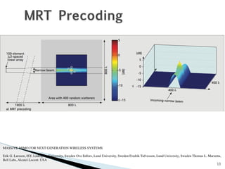
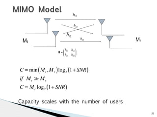
Download as PDF, PPTX
![8
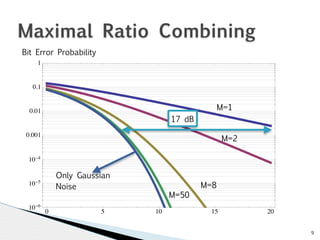
Bit Error Probability
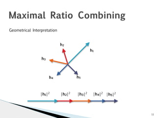
Maximal Ratio Combining
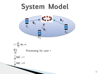
y = x + z
Pb = Q
2Eb
N0
⎛
⎝ ⎜
⎞
⎠ ⎟
y = [hhh!h]x + z
1 2 3M y = hx + z
h†y
MRC
M
Pb = 1
2
1− γ b
γ b + M
⎛
⎞
⎟
⎠ ⎜⎝ M −1+ k
M−1 Σ 1
k
⎛
⎝ ⎜
⎞
⎠ ⎟
k=0
2
+ 1
2
γ b
γ b + M
⎛
⎝ ⎜
⎞
⎠ ⎟
k
AWGN Channel
AWGN Channel
+Fading with
γ Diversity b = Eb
N0](https://image.slidesharecdn.com/channelmodelsformassivemimo-141202063750-conversion-gate01/85/Channel-Models-for-Massive-MIMO-8-320.jpg)

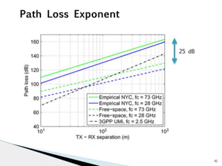
![36
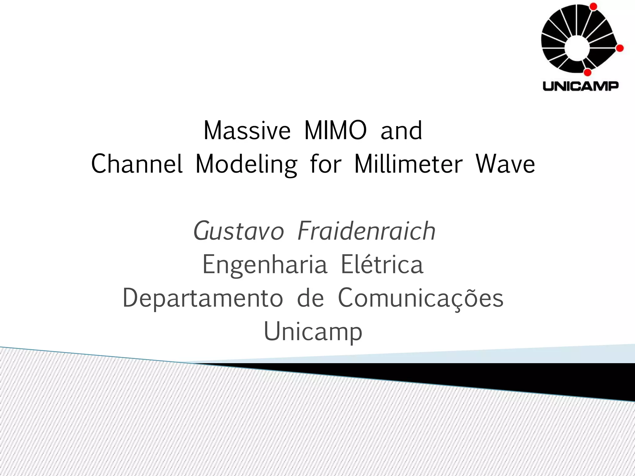
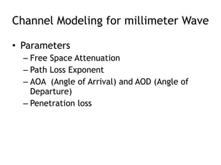
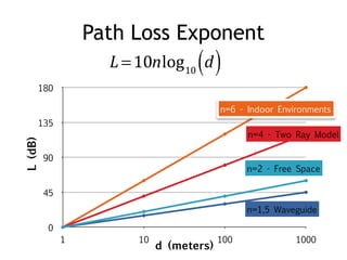
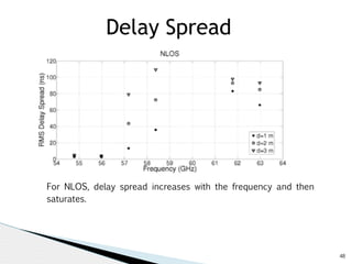
Path Loss Exponent
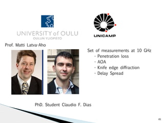
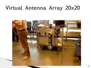
Frequency LOS NLOS Distance Reference
900 MHz 5.3 30-400 [7]
1800 MHz 5.5 30-400 [7]
2 GHz 1,56 1-20 [4]
2,3 GHz 6 30-400 [7]
5 GHz 1,87 1-20 [4]
17 GHz 1,98 1-20 [4]
28 GHz 2 2,92 30 — 200 [1]
28 GHZ 2,6 3,4 1—100 [2]
28 GHz 5,52 1-100 [9]
38 GHz 2.3 3.86 [10]
60 GHz 1,52 0,5 — 3 [5]
73 GHz 2 2,57 30 — 200 [1]
73 GHz 2 3,4 1—100 [2]](https://image.slidesharecdn.com/channelmodelsformassivemimo-141202063750-conversion-gate01/85/Channel-Models-for-Massive-MIMO-36-320.jpg)
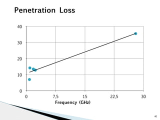
![39
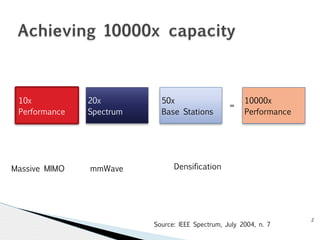
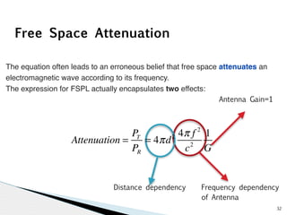
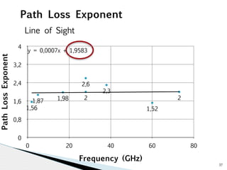
Penetration Loss
Frequency Loss (dB) Material Reference
800 MHz 7 Wall [6]
900 MHz 14,2 Wall [7]
1.8 GHz 13,5 Wall [3]
1,8 GHz 13,4 Wall [7]
2,3 GHz 12,8 Wall [7]
28 GHz 35,5 Wall [8]](https://image.slidesharecdn.com/channelmodelsformassivemimo-141202063750-conversion-gate01/85/Channel-Models-for-Massive-MIMO-39-320.jpg)

![58
References
[1] - Mustafa Riza Akdeniz, Yuanpeng Liu, Mathew K. Samimi, Shu Sun, Student Member, IEEE, Sundeep Rangan,
Theodore S. Rappaport, and Elza Erkip, "Millimeter Wave Channel Modeling and Cellular Capacity Evaluation,”, IEEE
JOURNAL ON SELECTED AREAS IN COMMUNICATIONS, VOL. 32, NO. 6, JUNE 2014.
[2] - Millimeter Wave Cellular Ultra-Wideband Statistical Channel Model for NonLine of Sight Millimeter-Wave Urban
Channels Communications: Channel Models, Capacity Limits, Challenges and Opportunities
Prof. Ted Rappaport NYU WIRELESS, NYU Polytechnic School of Engineering, Joint work with Sundeep Rangan and Elza
Erkip.
[3] - A. F. Toledo, D. GJ Lewis, and A.M.D. Turkmani, "Radio Propagation into Buildings at 1.8 GHz”
[4] P. Nobles, and F. Halsall, "Delay Spread and Received Power Measurements within a Building at 2GHz, 5 GHz and 17
Ghz,”
[5] - Maria-Teresa Martinez-Ingles, Davy P. Gaillot, Juan Pascual-Garcia, Jose-Maria Molina-Garcia-Pardo, Martine Lienard,
and José-Víctor Rodríguez, “Deterministic and Experimental Indoor mmW Channel Modeling, “IEEE ANTENNAS AND
WIRELESS PROPAGATION LETTERS, VOL. 13, 2014 1047.
[6] -D. Cox, "Measurements of 800 MHz Radio Transmission
Into Buildings with Metallic Walls”, The Bell System Technical Journal 1983
[7] - A. F. Toledo, , Adel Turlmani, and David Parsons, "Estimating Coverage of Radio Transmission into and within
Buildings at 900, 1800, and 2300 MHz,” IEEE Personal Communications April 1998.
[8] - Hao Xu, Member, IEEE, Vikas Kukshya, Member, IEEE, and Theodore S. Rappaport, Fellow, IEEE , “Spatial and
Temporal Characteristics of 60-GHz Indoor Channels, “IEEE JOURNAL ON SELECTED AREAS IN COMMUNICATIONS, VOL.
20, NO. 3, APRIL 2002.
[9] - Mathew Samimi, Kevin Wang, Yaniv Azar, George N. Wong, Rimma Mayzus, Hang Zhao, Jocelyn K. Schulz, Shu Sun,
Felix Gutierrez, Jr., and Theodore S. Rappaport , 28 GHz Angle of Arrival and Angle of Departure Analysis for Outdoor
Cellular Communications using Steerable Beam Antennas in New York City, VTC 2013.
[10] - Theodore S. Rappaport, Yijun Qiao, Jonathan I. Tamir, James N. Murdock, Eshar Ben-Dor , “Cellular Broadband
Millimeter Wave Propagation and Angle of Arrival for Adaptive Beam Steering Systems (Invited Paper),”RWS 2012.
[11] - Dajana Cassioli, Luca Alfredo Annoni and Stefano Piersanti, “Characterization of Path Loss and Delay Spread of 60-
GHz UWB Channels vs. Frequency, “ IEEE ICC 2013 - Wireless Communications Symposium.](https://image.slidesharecdn.com/channelmodelsformassivemimo-141202063750-conversion-gate01/85/Channel-Models-for-Massive-MIMO-58-320.jpg)


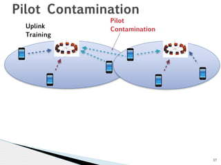
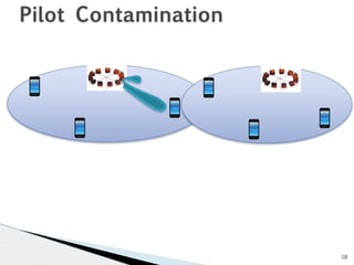
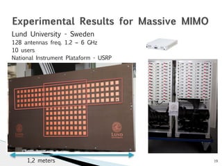
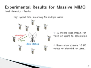
The document discusses the concept of massive MIMO (Multiple Input Multiple Output) systems and their application in millimeter wave communication. It highlights how such systems can achieve significant performance improvements through large antenna arrays at base stations, allowing for simultaneous user servicing and improved channel modeling. Additionally, it addresses challenges like pilot contamination and penetration loss, stressing the need for advanced channel modeling techniques in next-generation wireless systems.


![Getting Started with Apache Spark: Big Data Made Simple [Free Meetup]](https://cdn.slidesharecdn.com/ss_thumbnails/apachesparkgettingstarted-260203175547-8361bcc3-thumbnail.jpg?width=640&height=640&fit=bounds)


