Downloaded 86 times
![GIS for Drainage Assessment Andrew Harrison, GISP Business Development Manager The Schneider Corporation (317) 826-7393 [email_address]](https://image.slidesharecdn.com/watersheddraincalcicit-111011175215-phpapp01/75/Watershed-development-and-drainage-assessments-1-2048.jpg)

![Thank you! Presenter: Andrew Harrison, GISP Business Development Manager The Schneider Corporation (317) 826-7393 [email_address]](https://image.slidesharecdn.com/watersheddraincalcicit-111011175215-phpapp01/75/Watershed-development-and-drainage-assessments-47-2048.jpg)

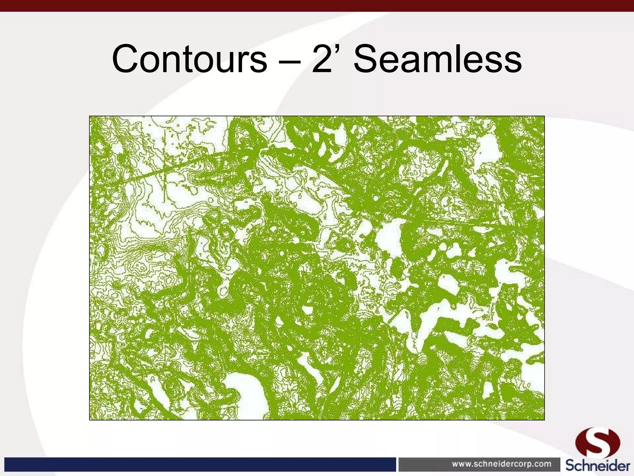
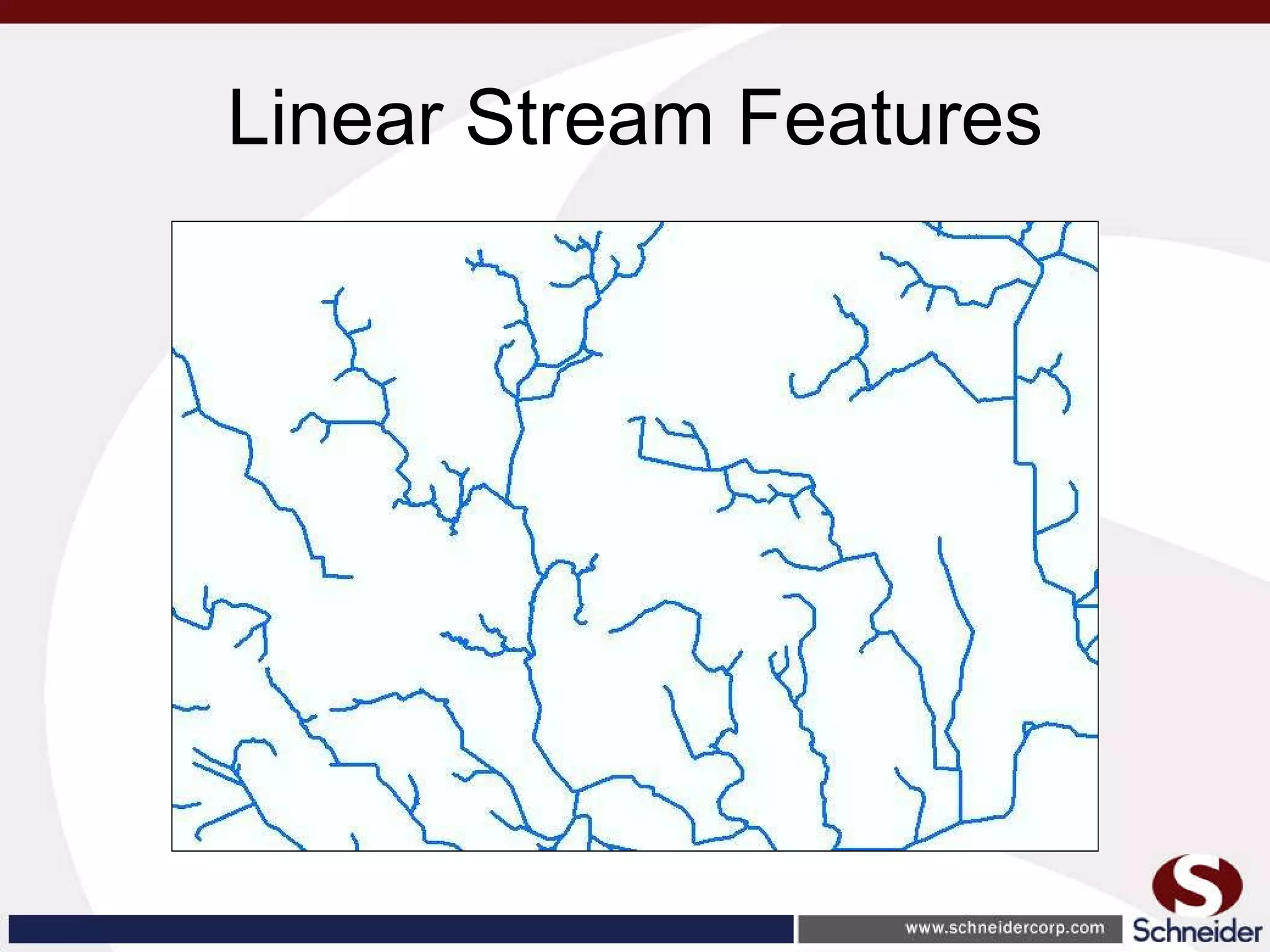
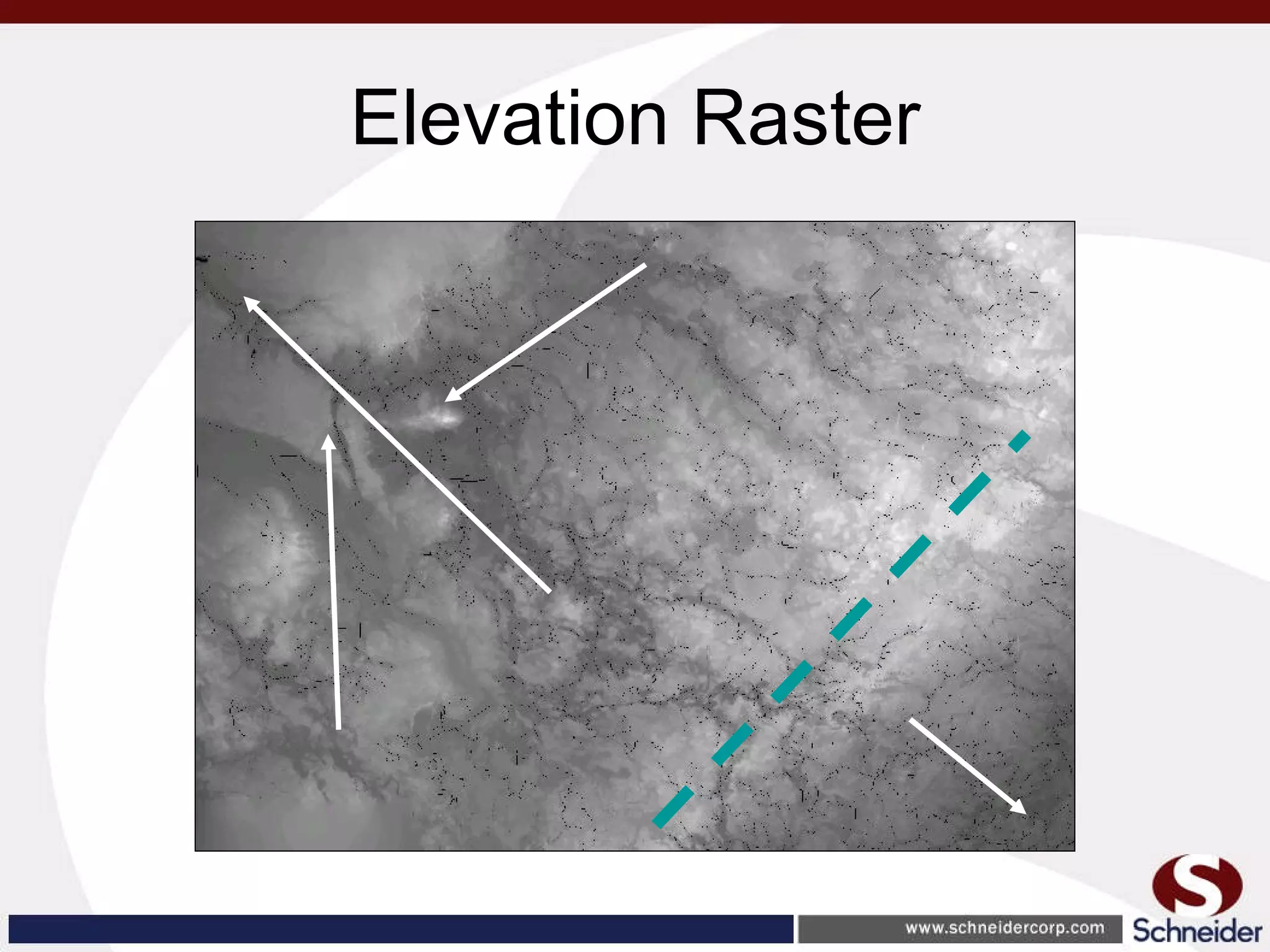
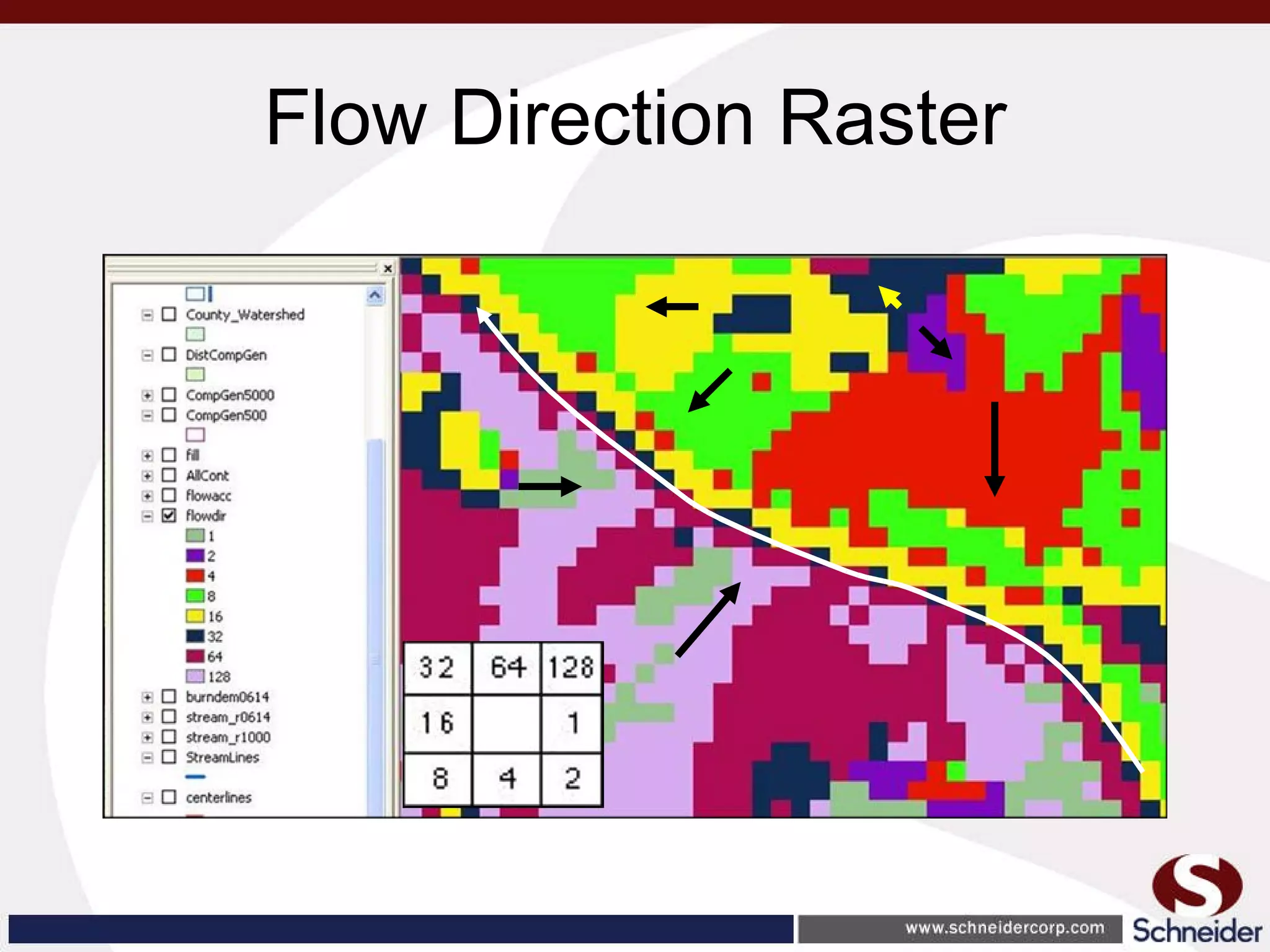
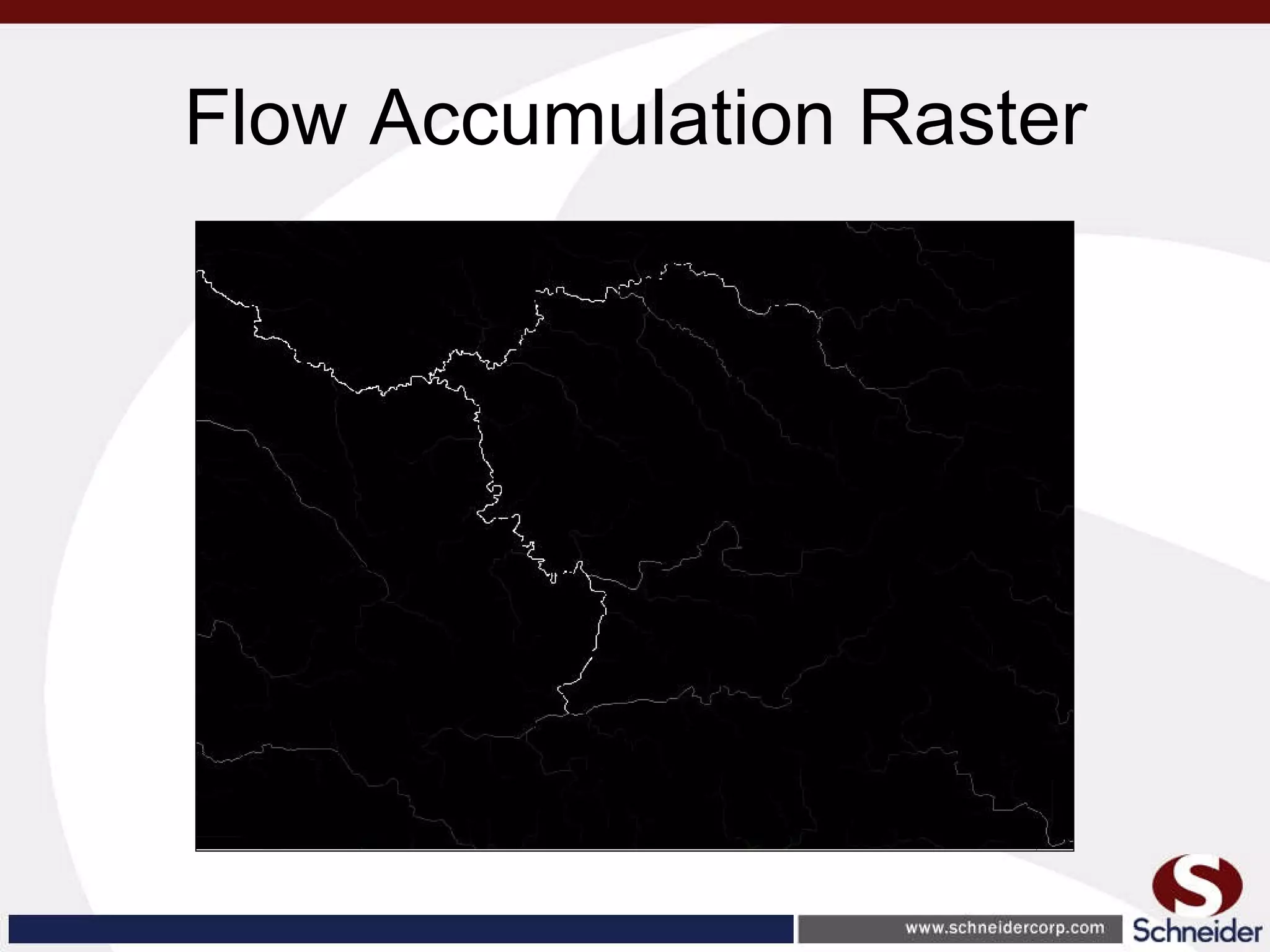
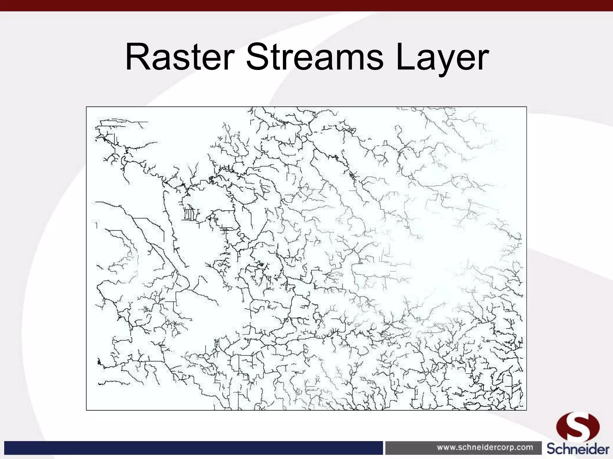
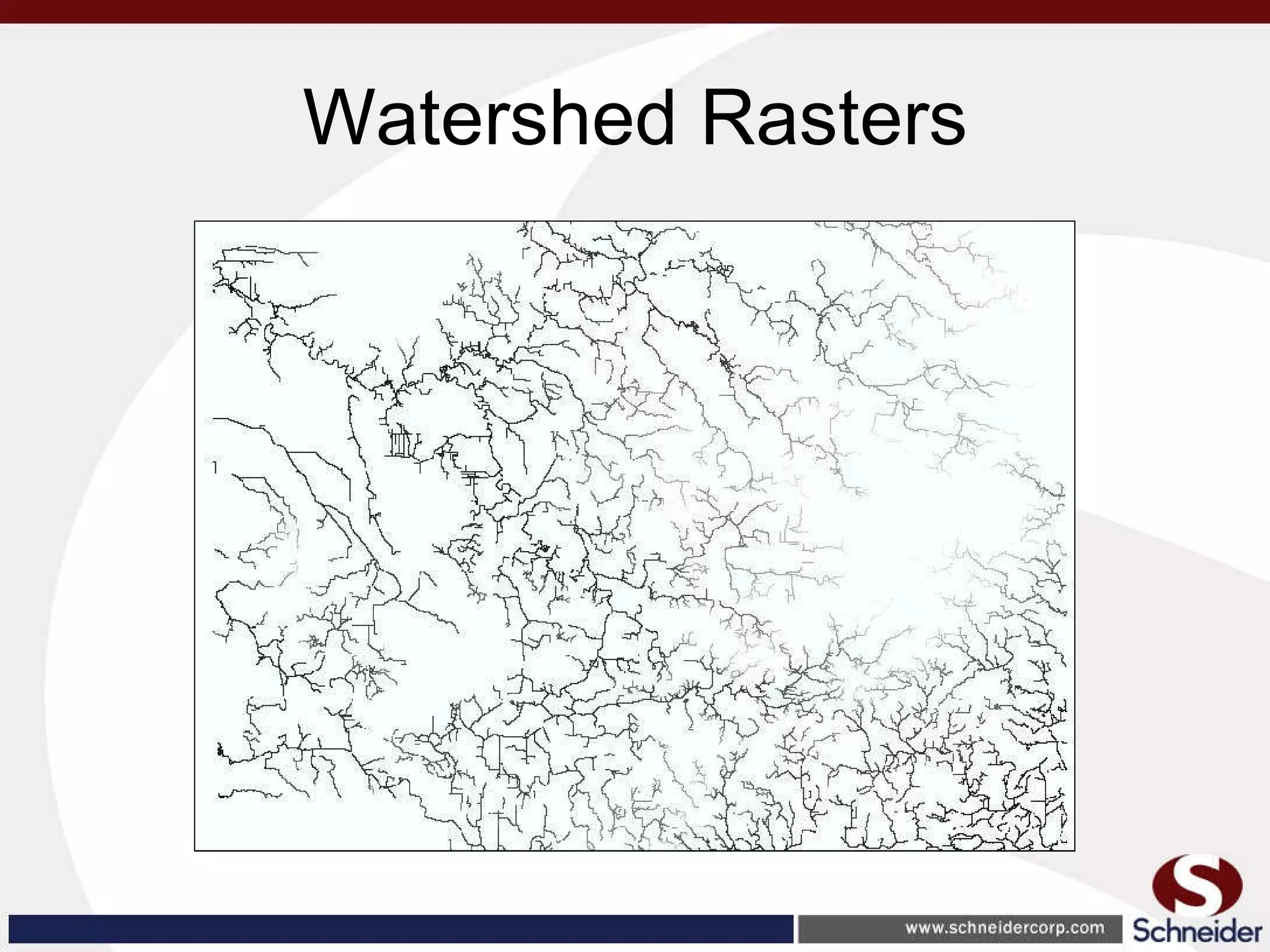
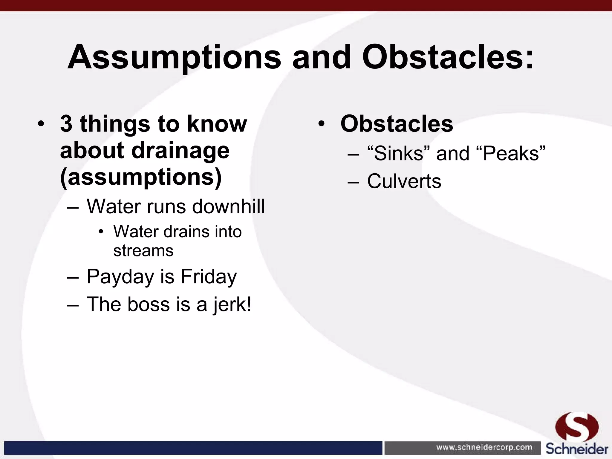
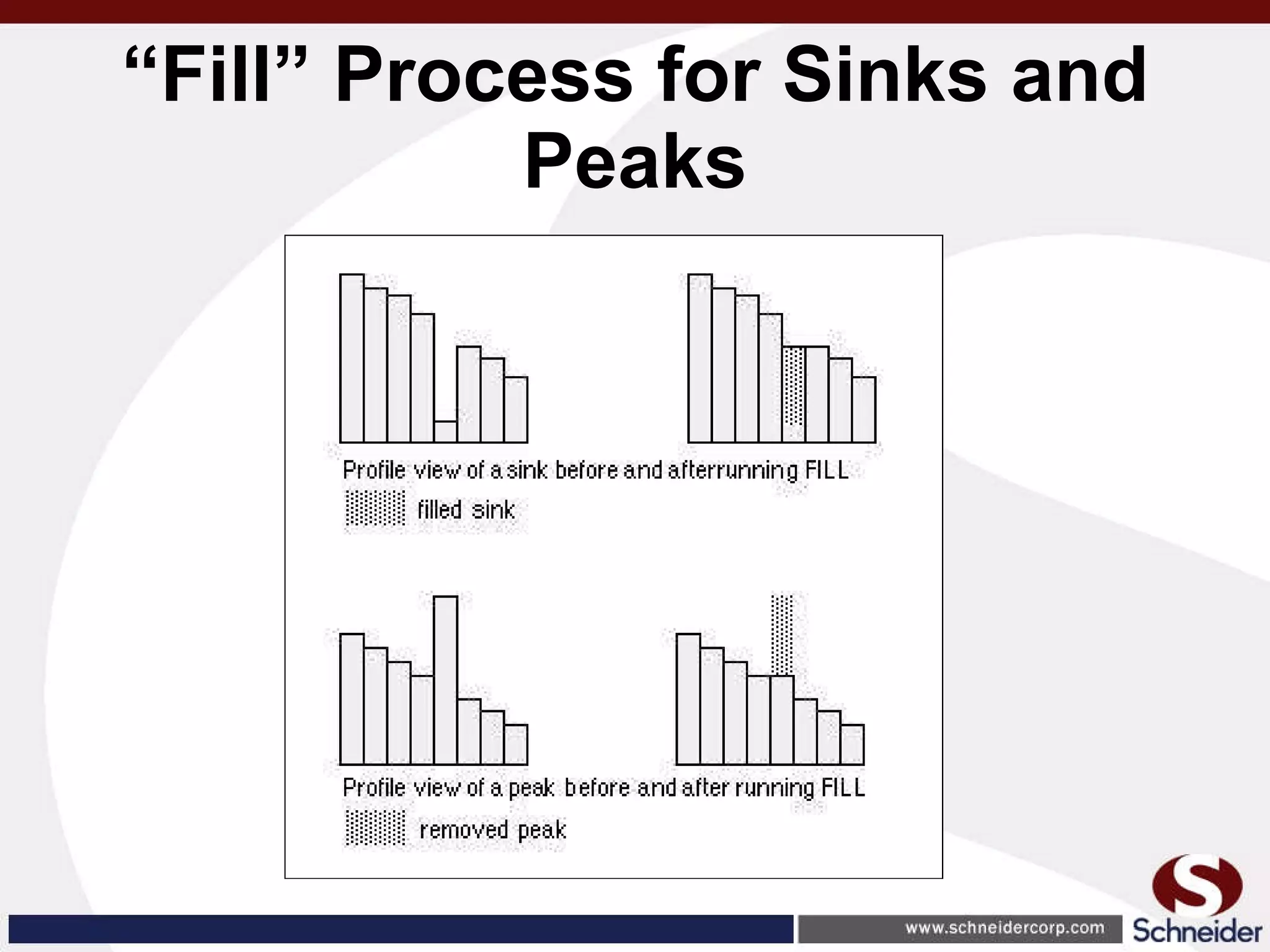
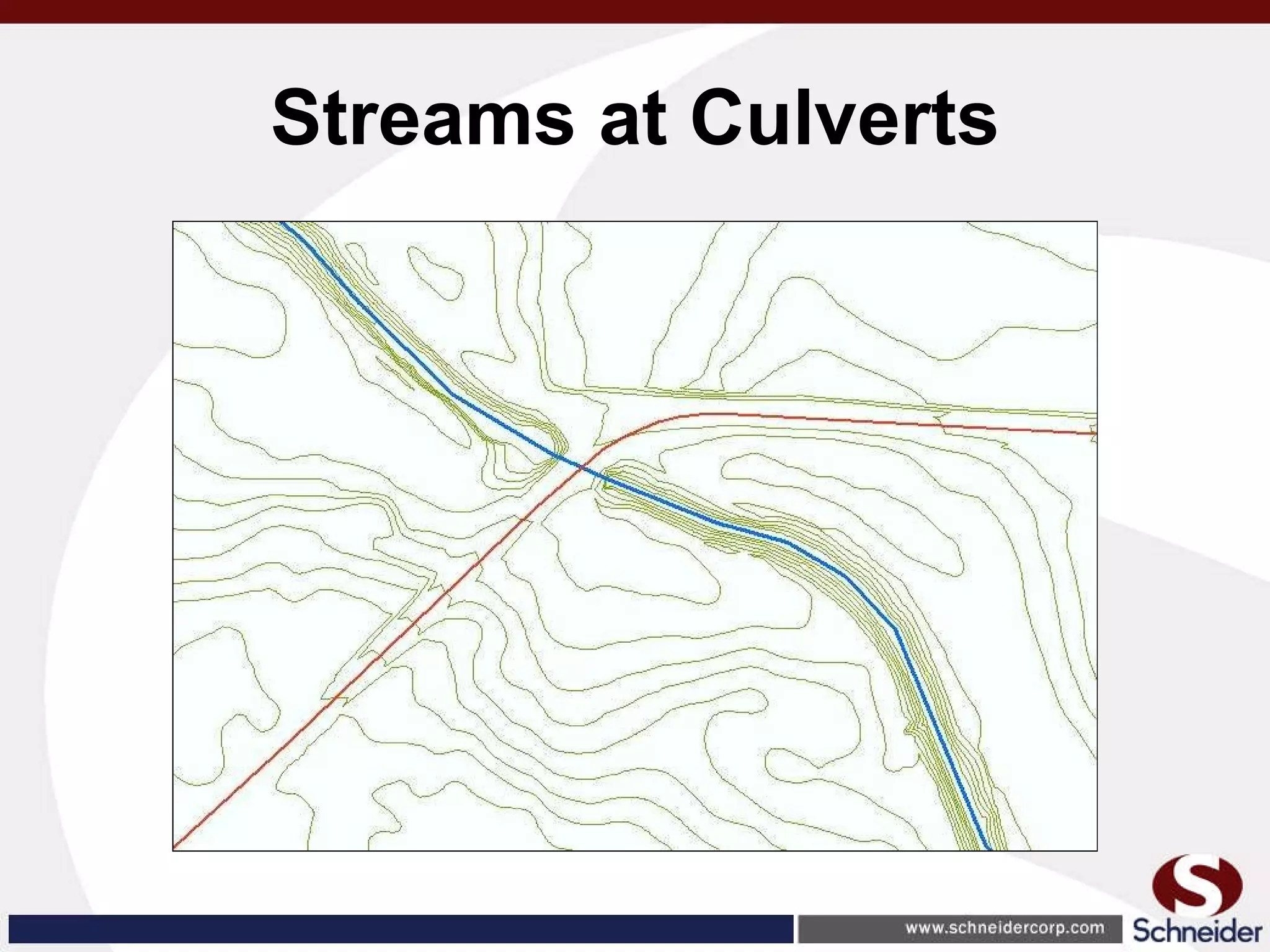
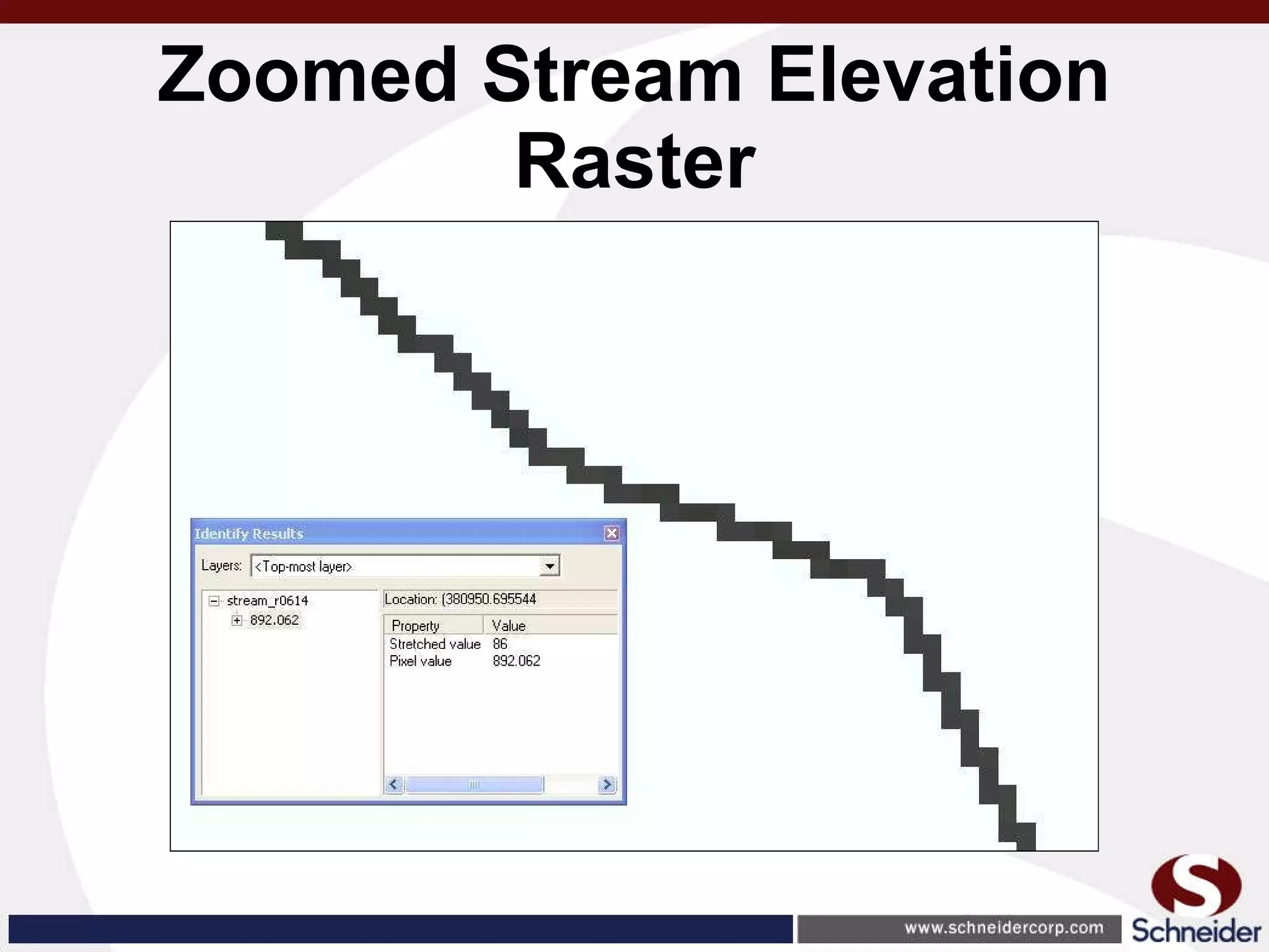
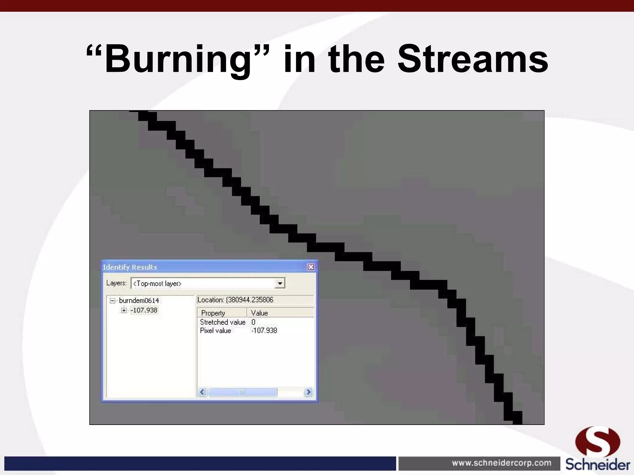
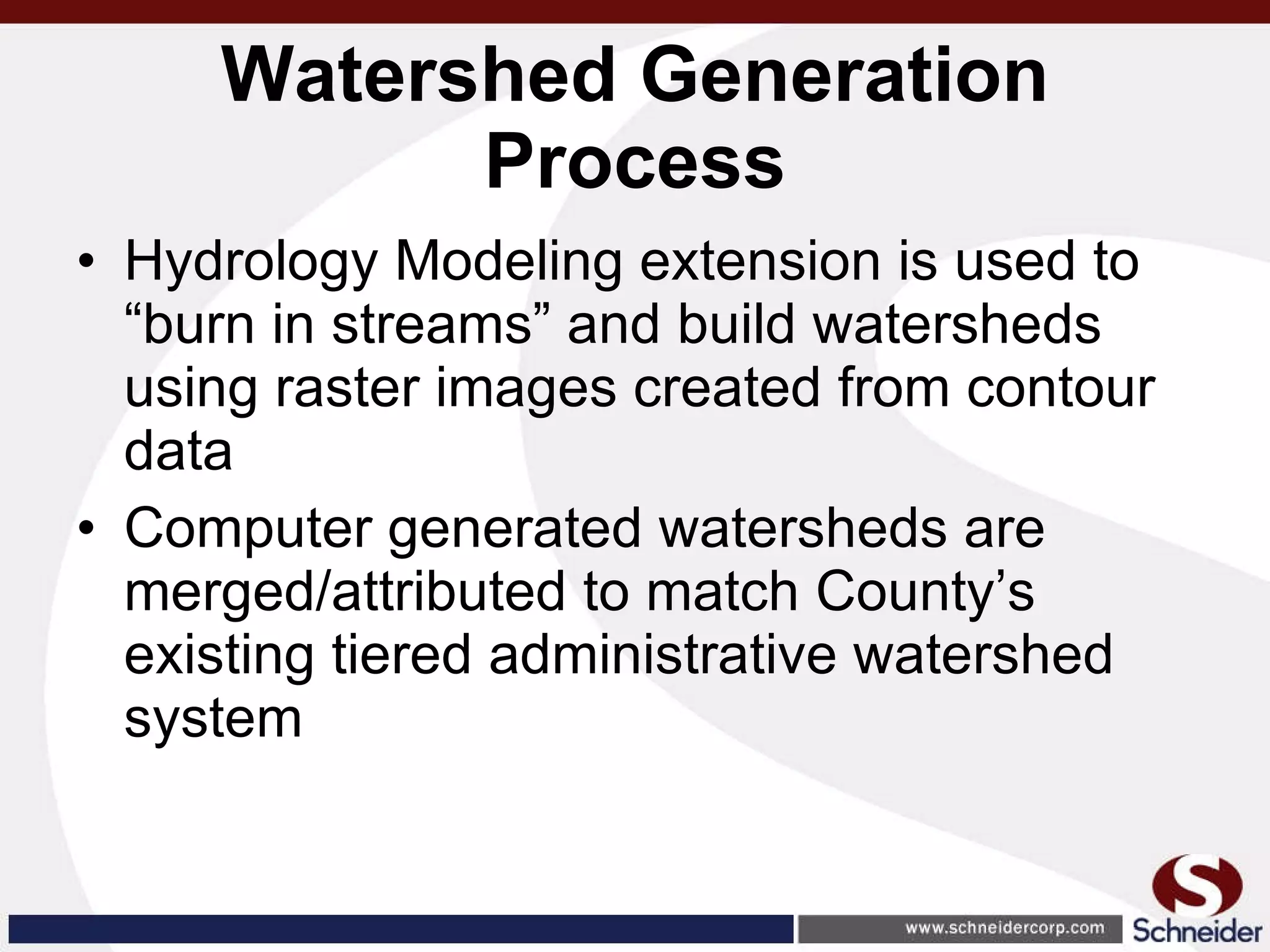
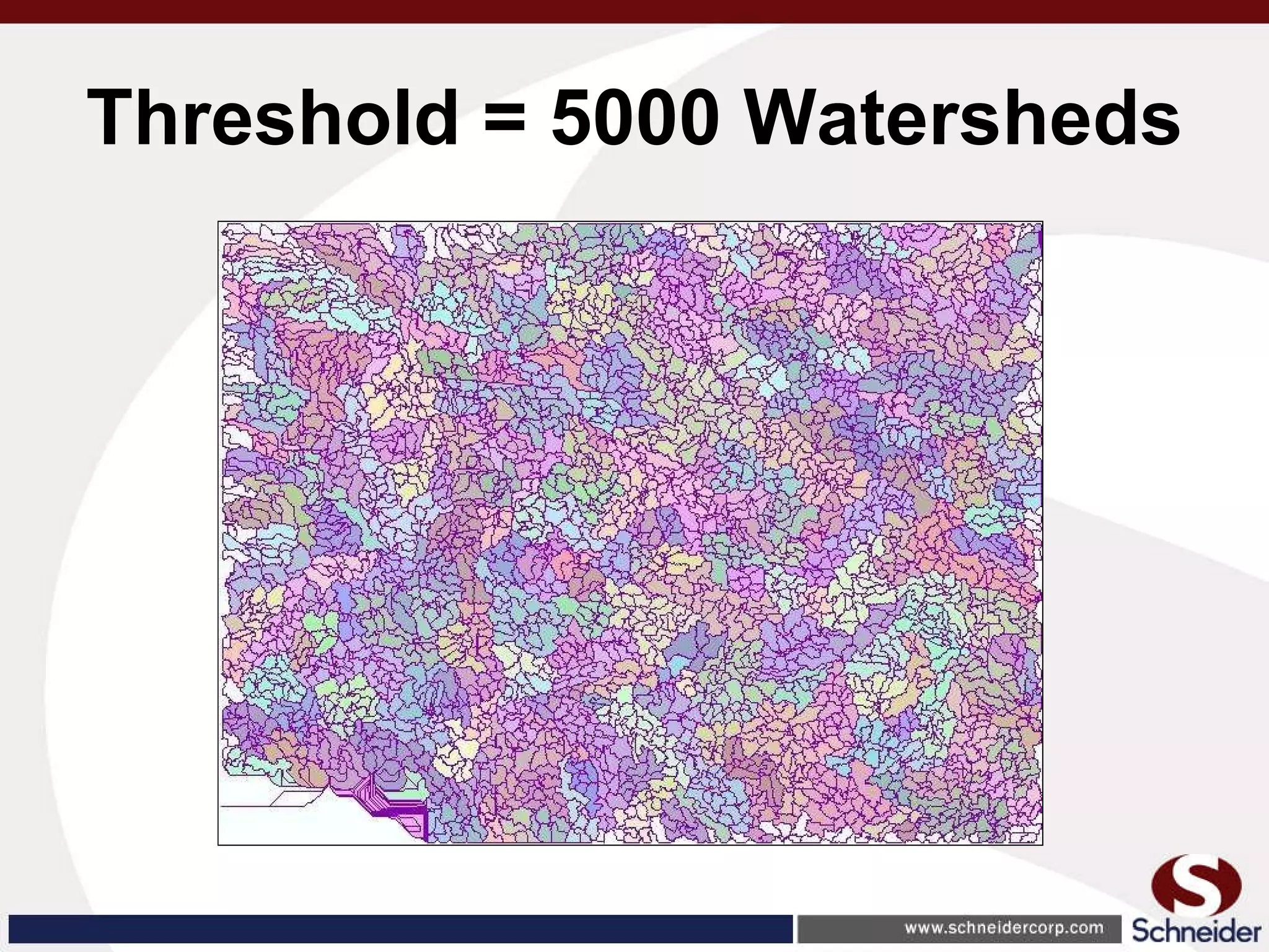
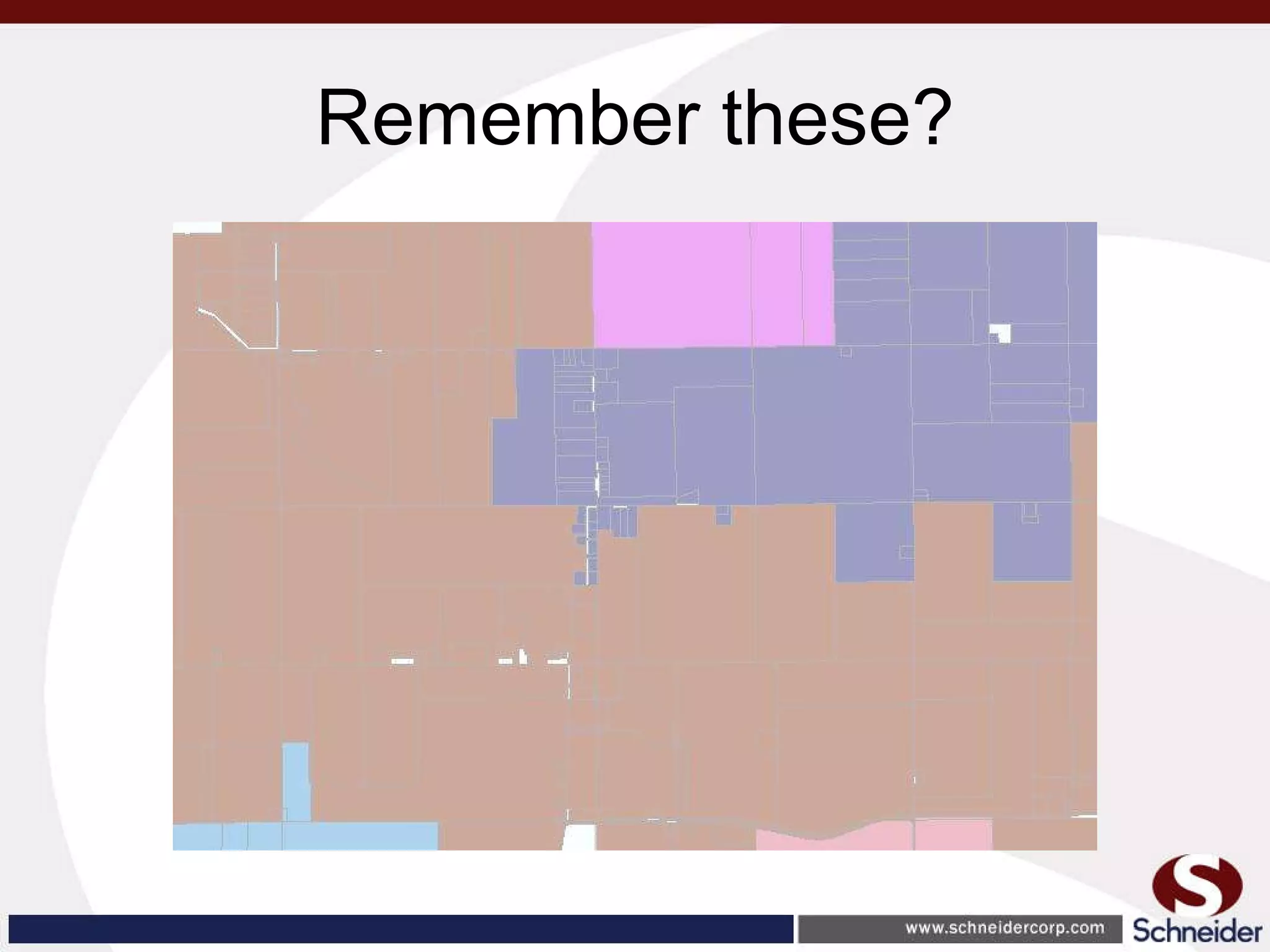
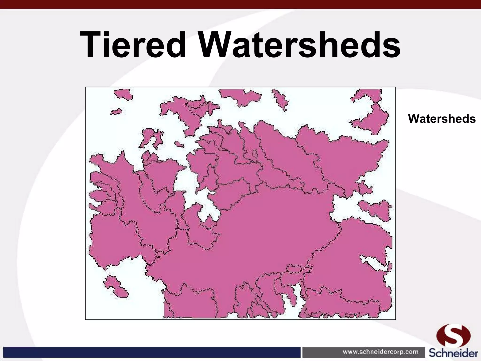
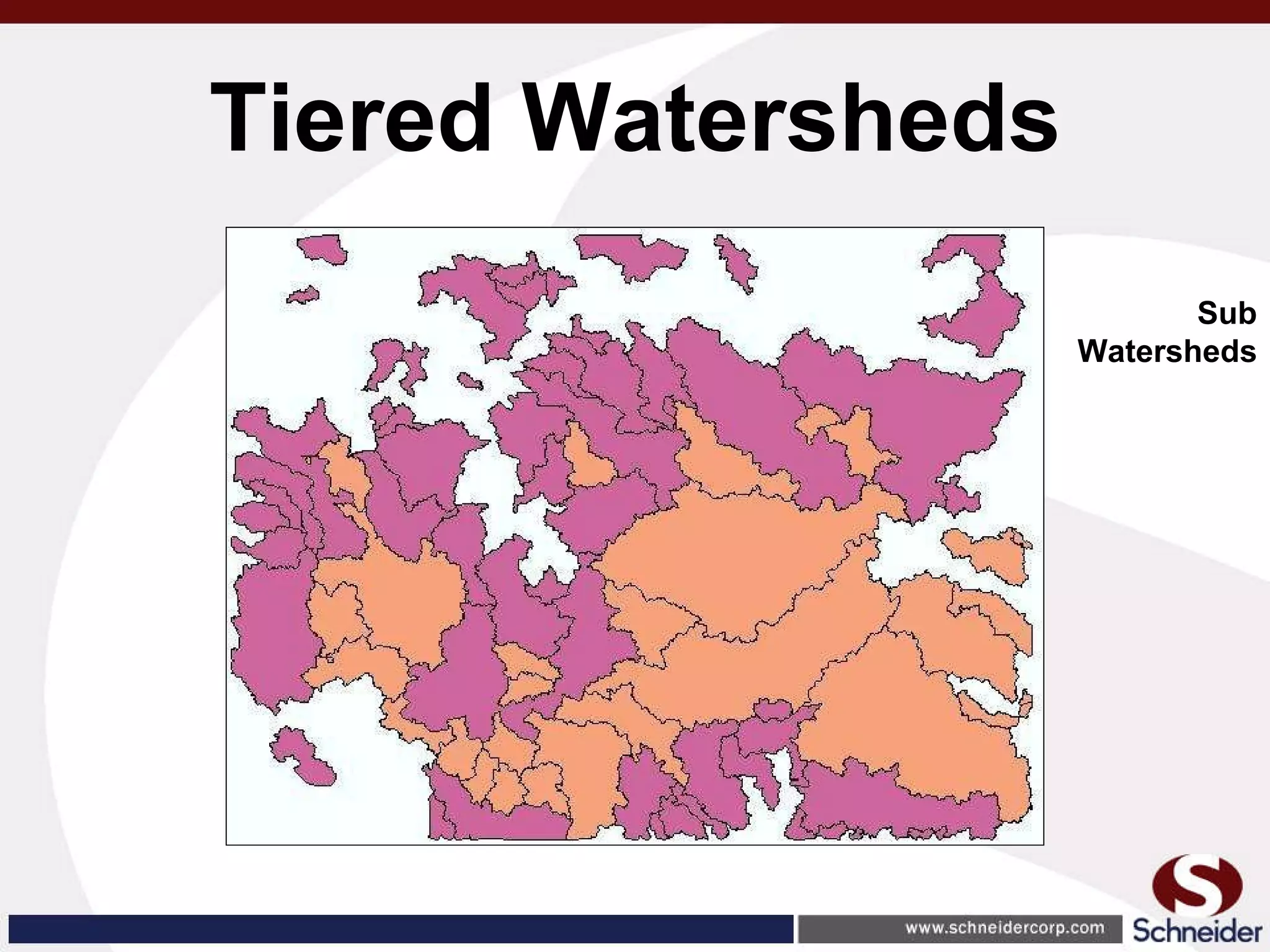
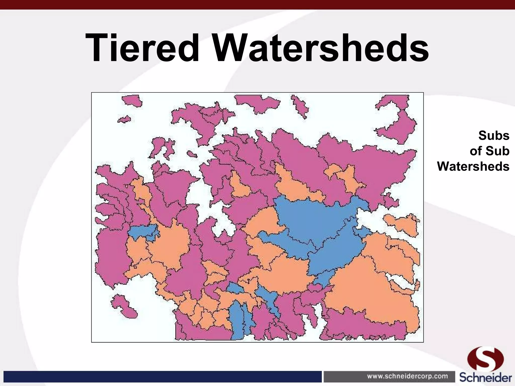
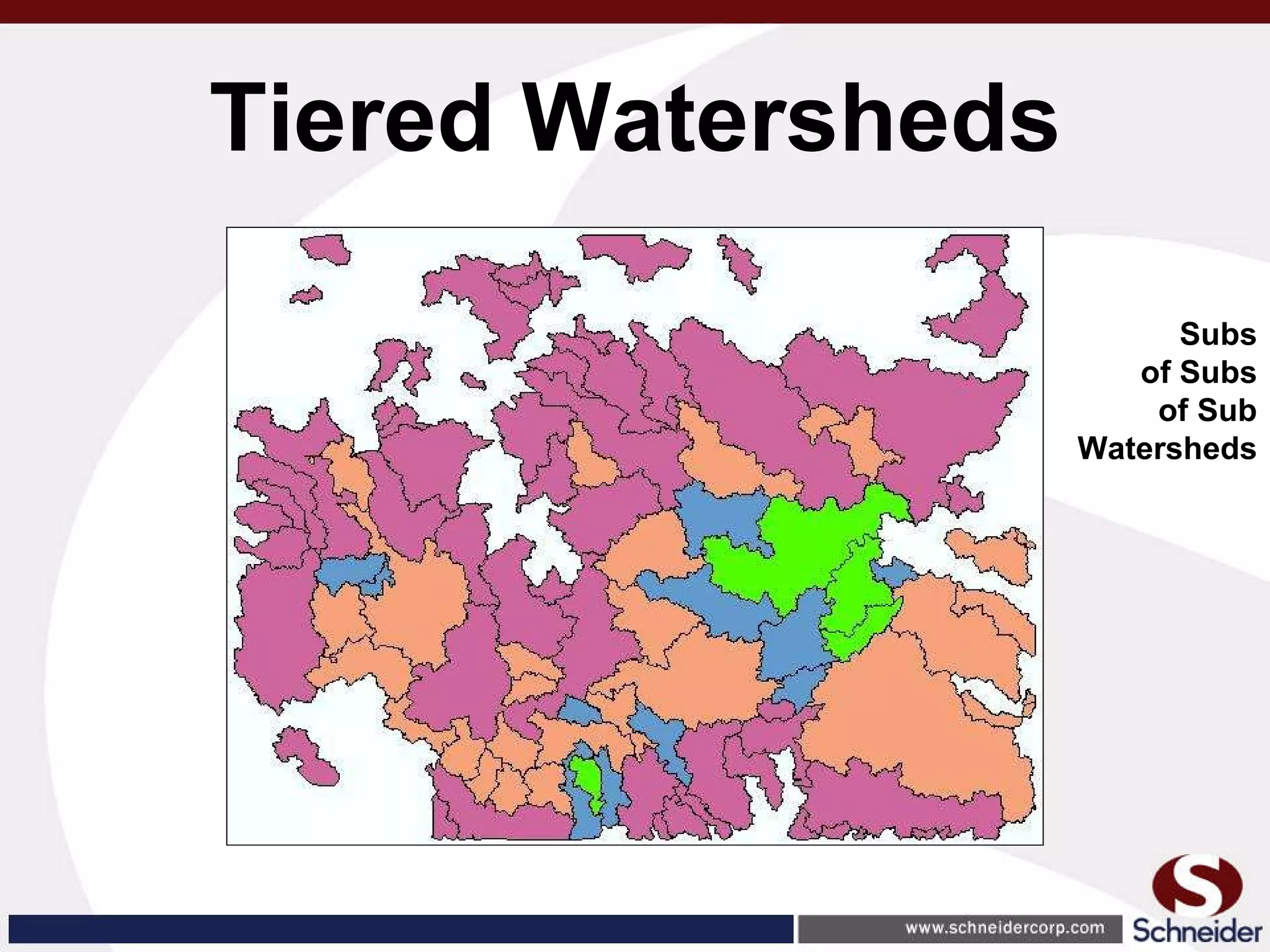
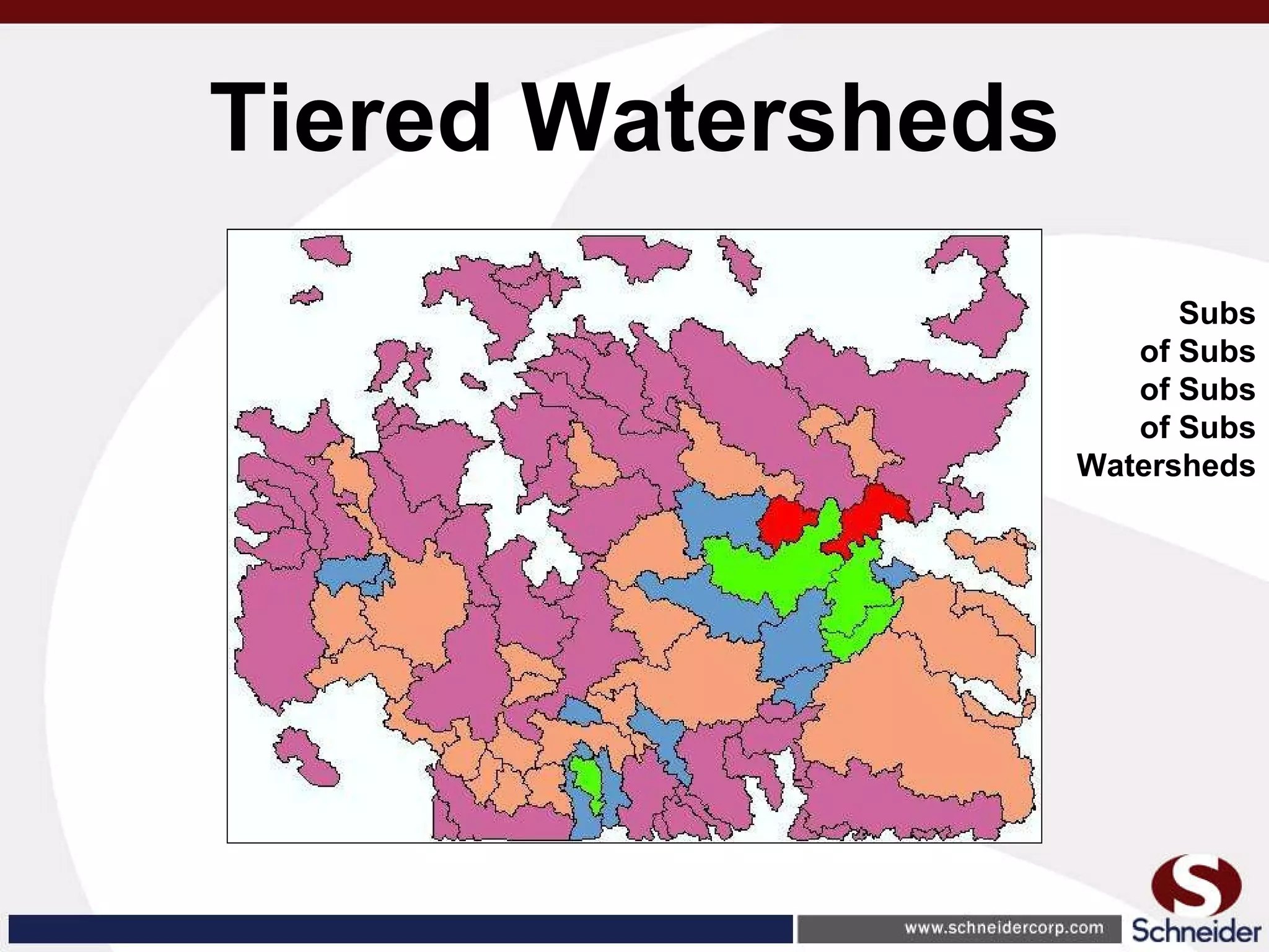
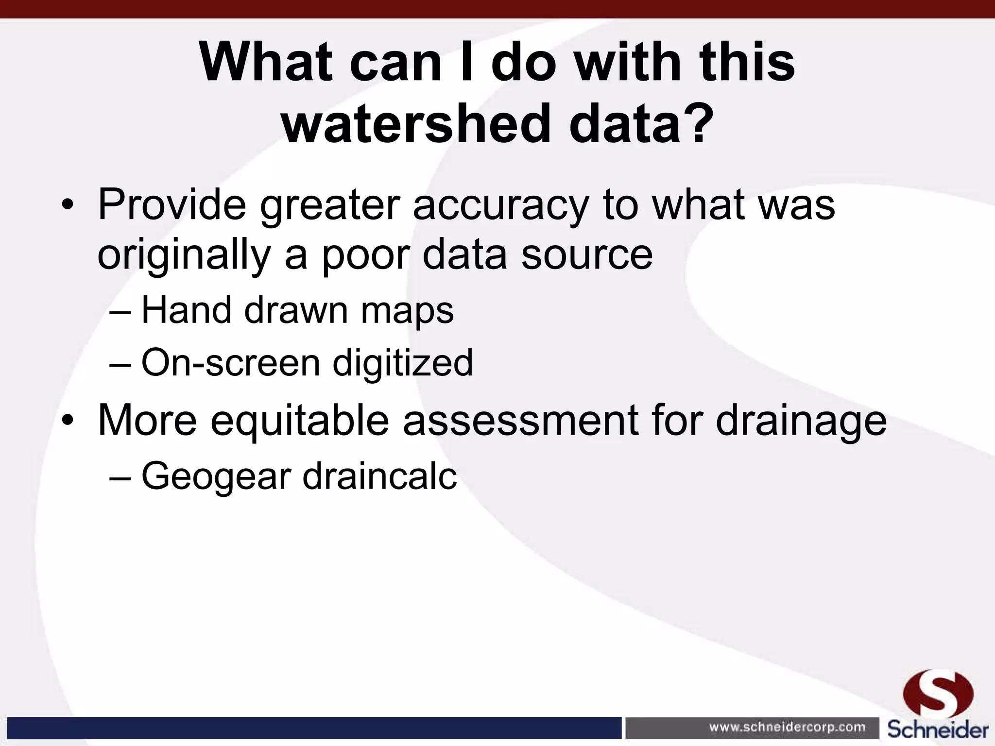
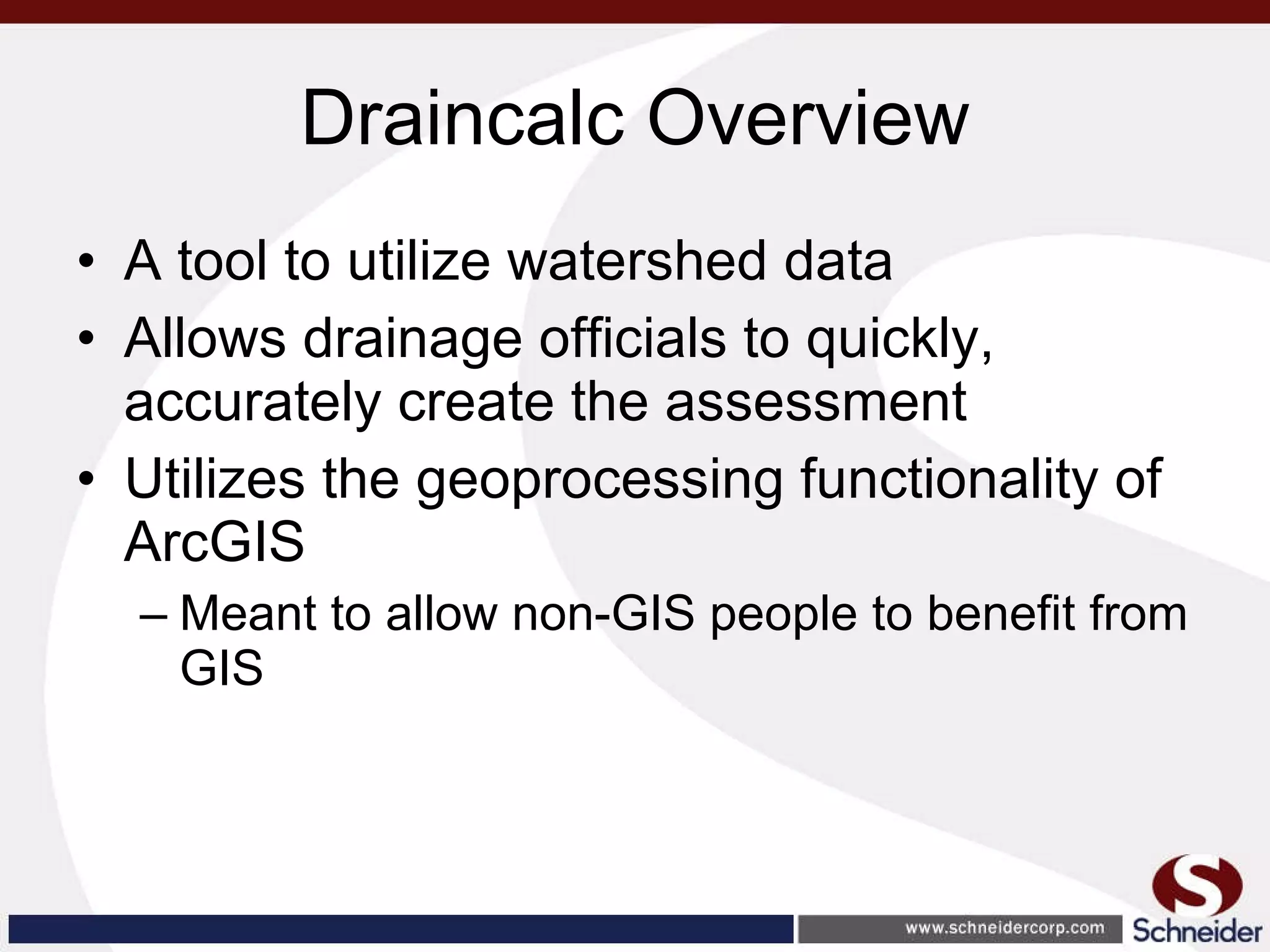
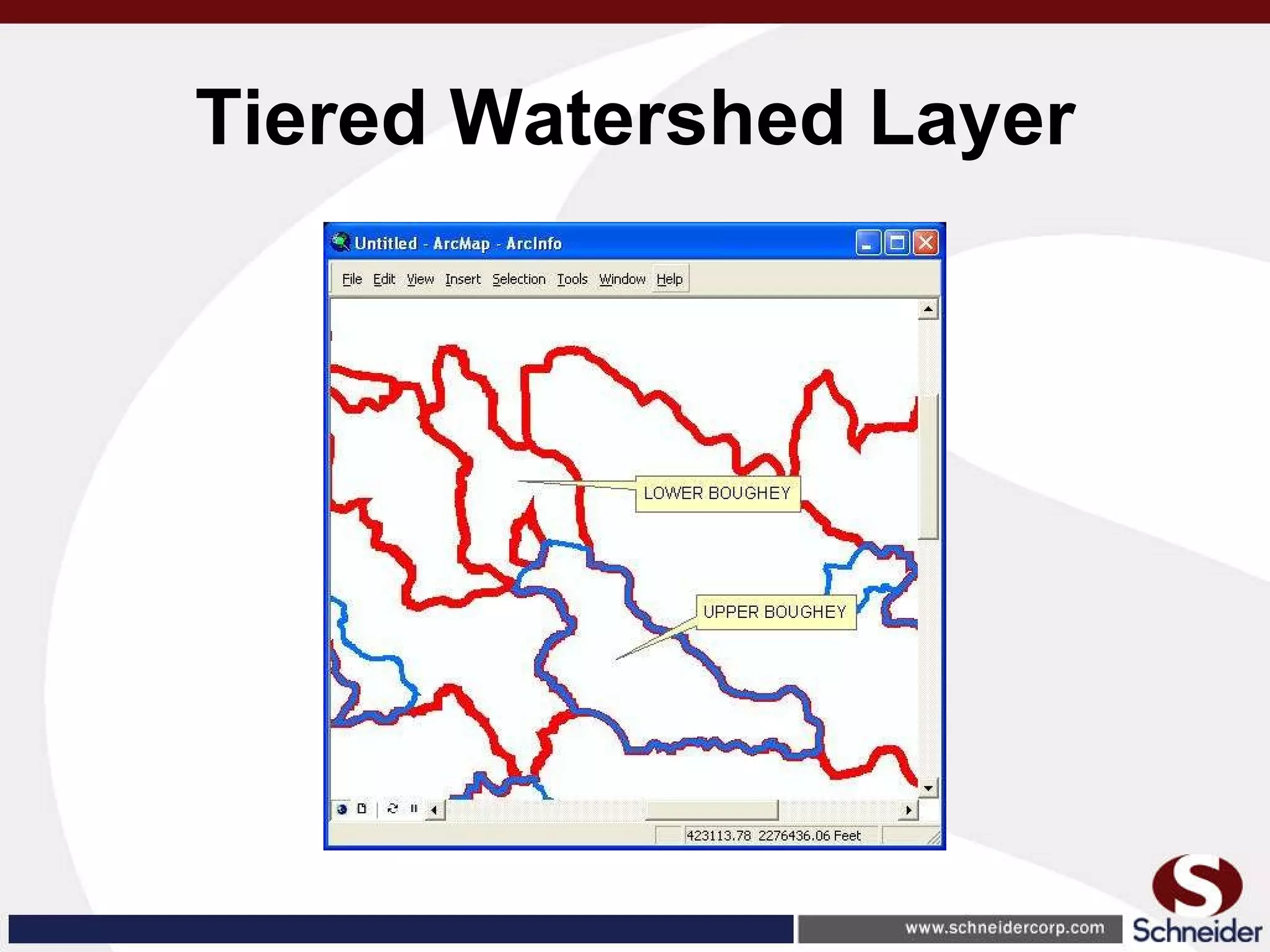
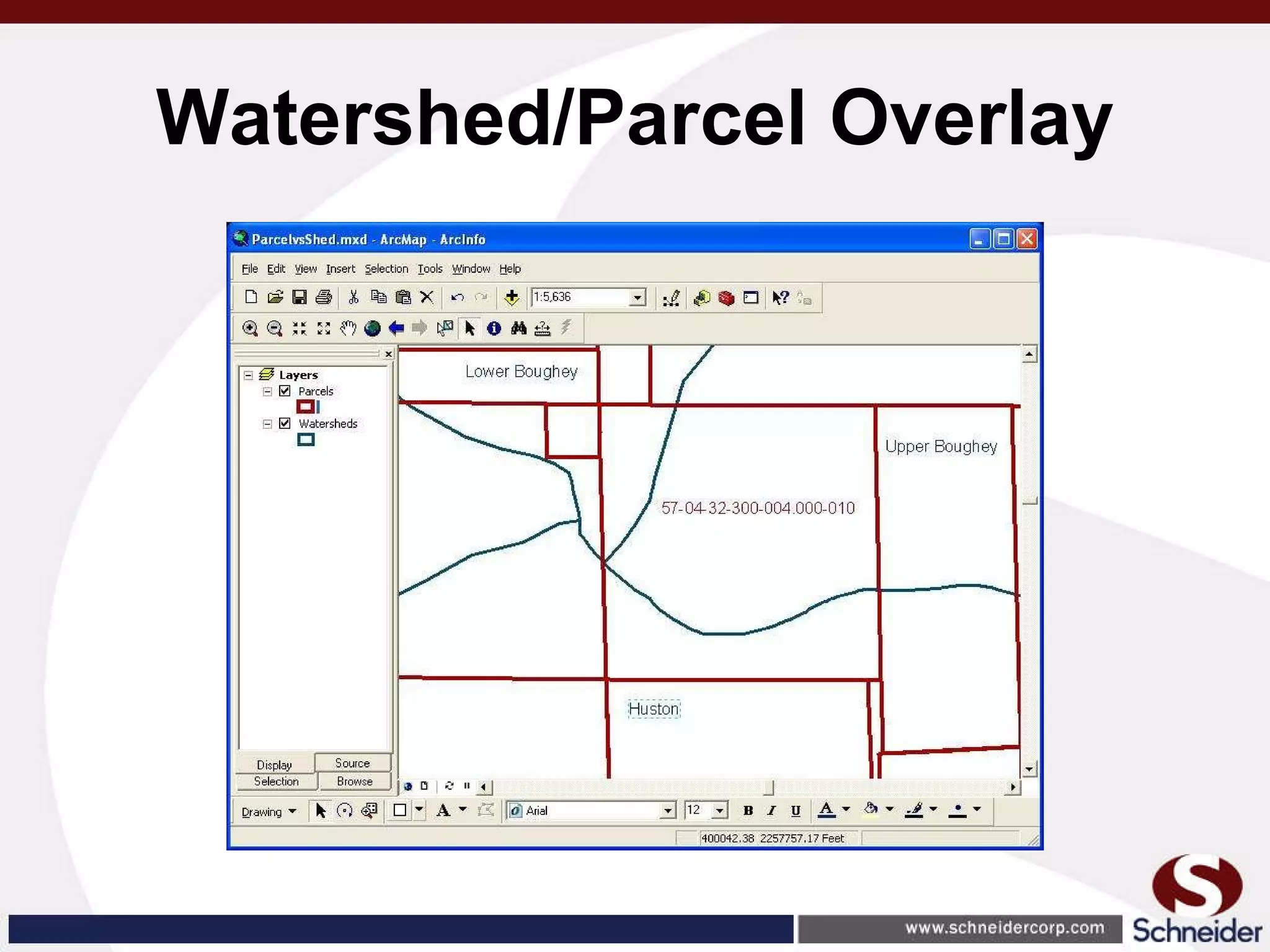
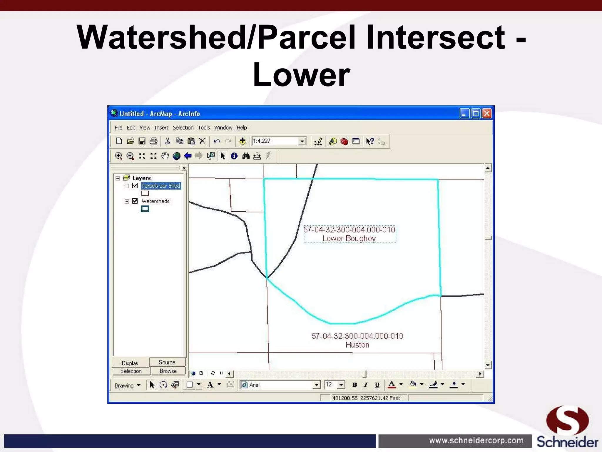
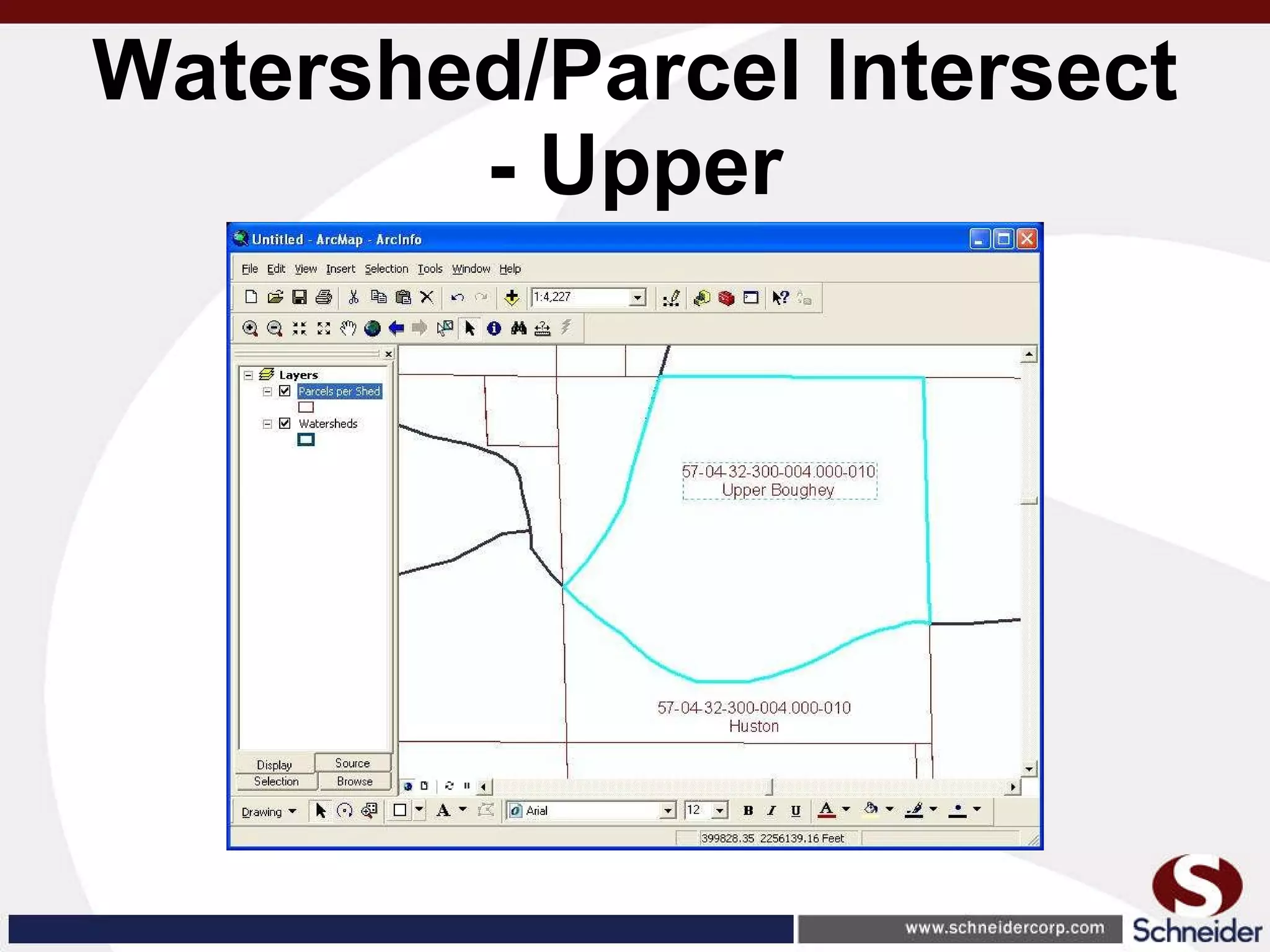
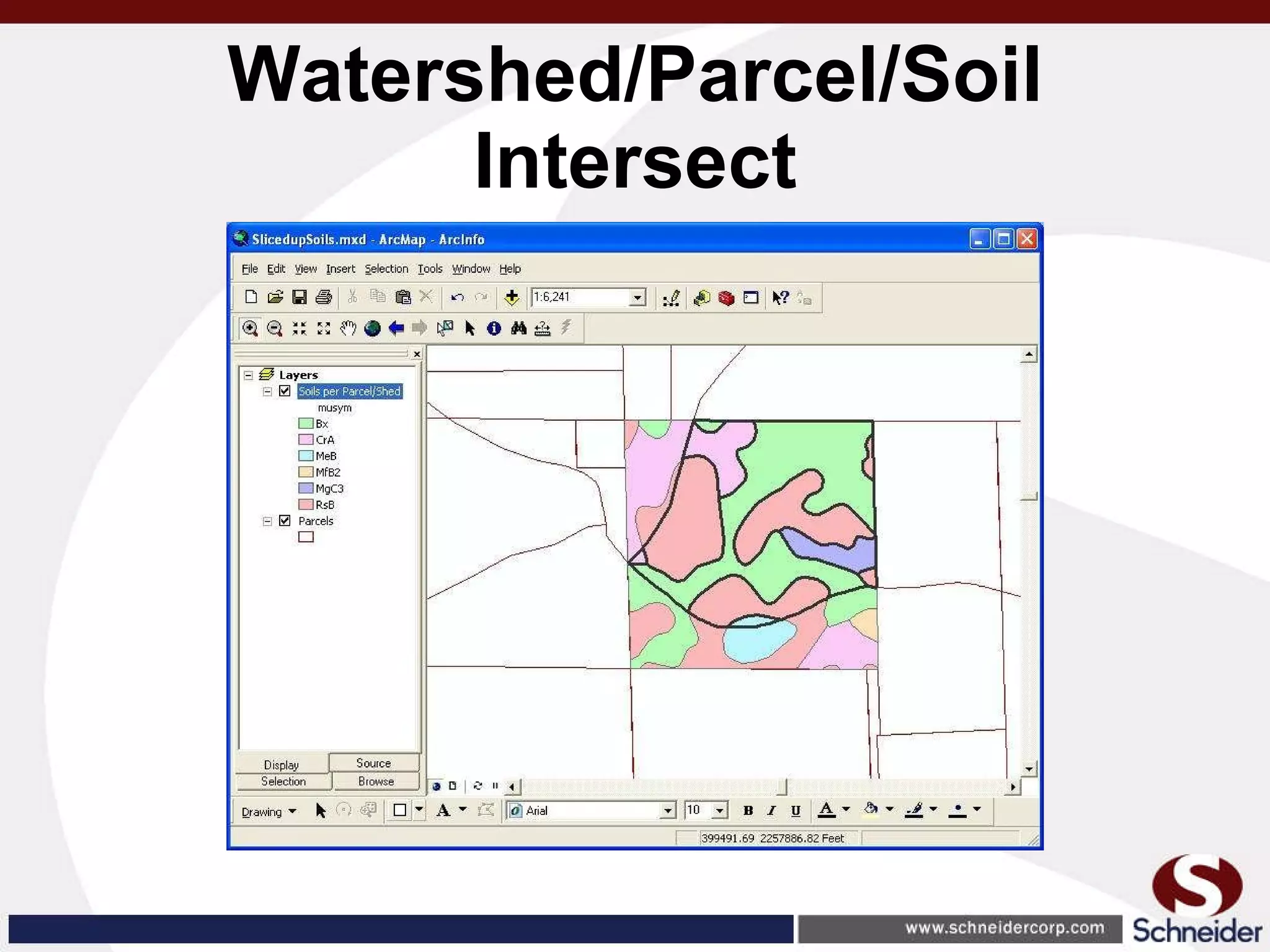
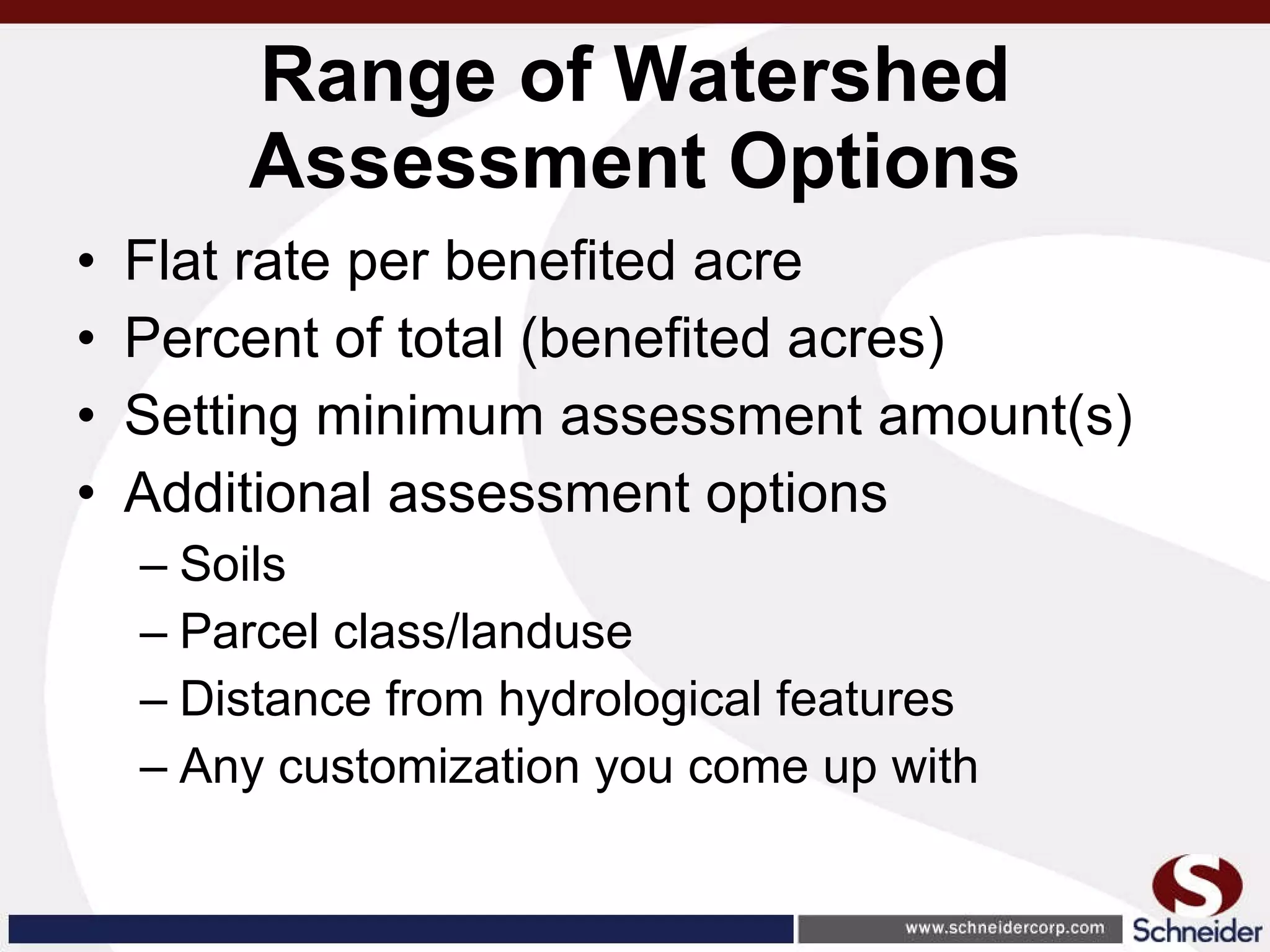
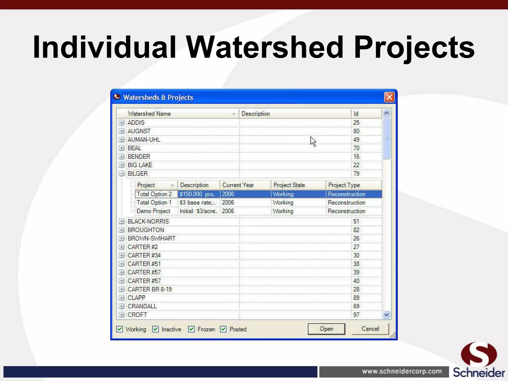
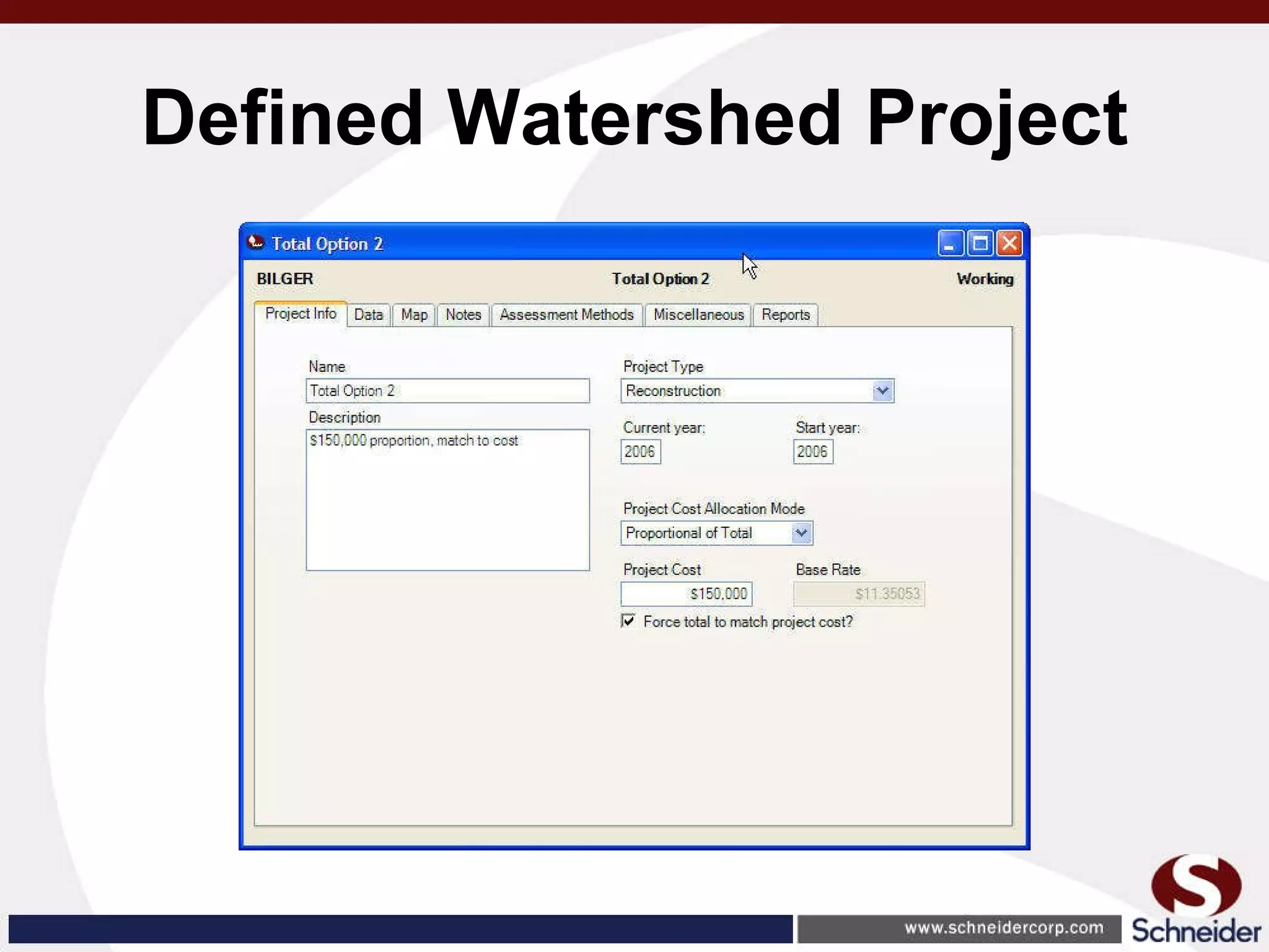
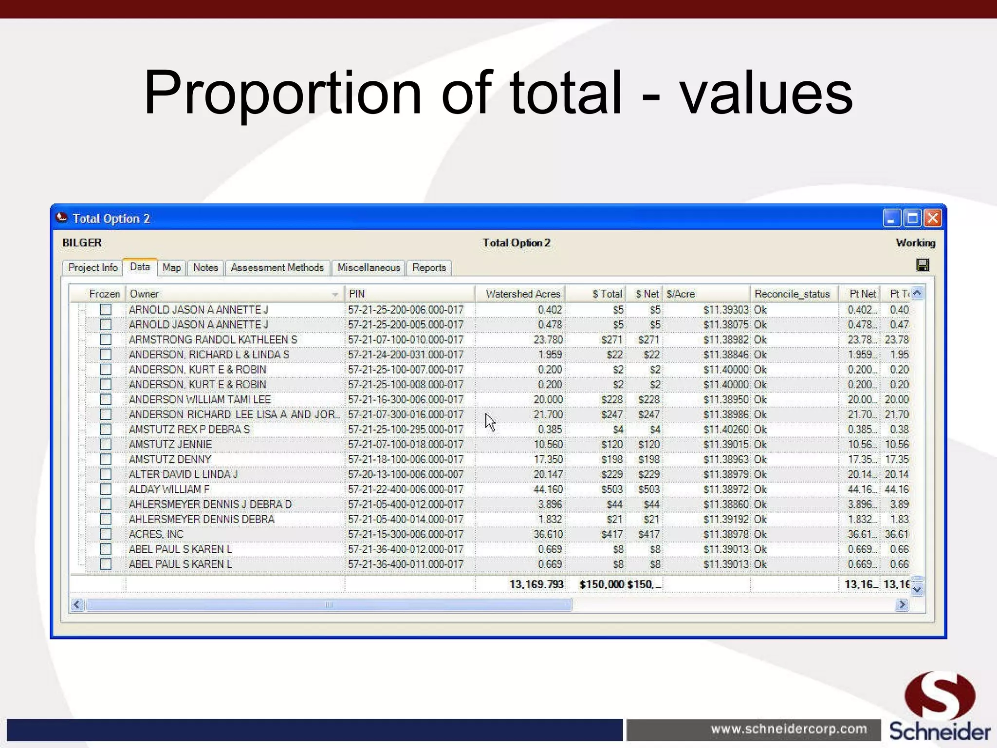
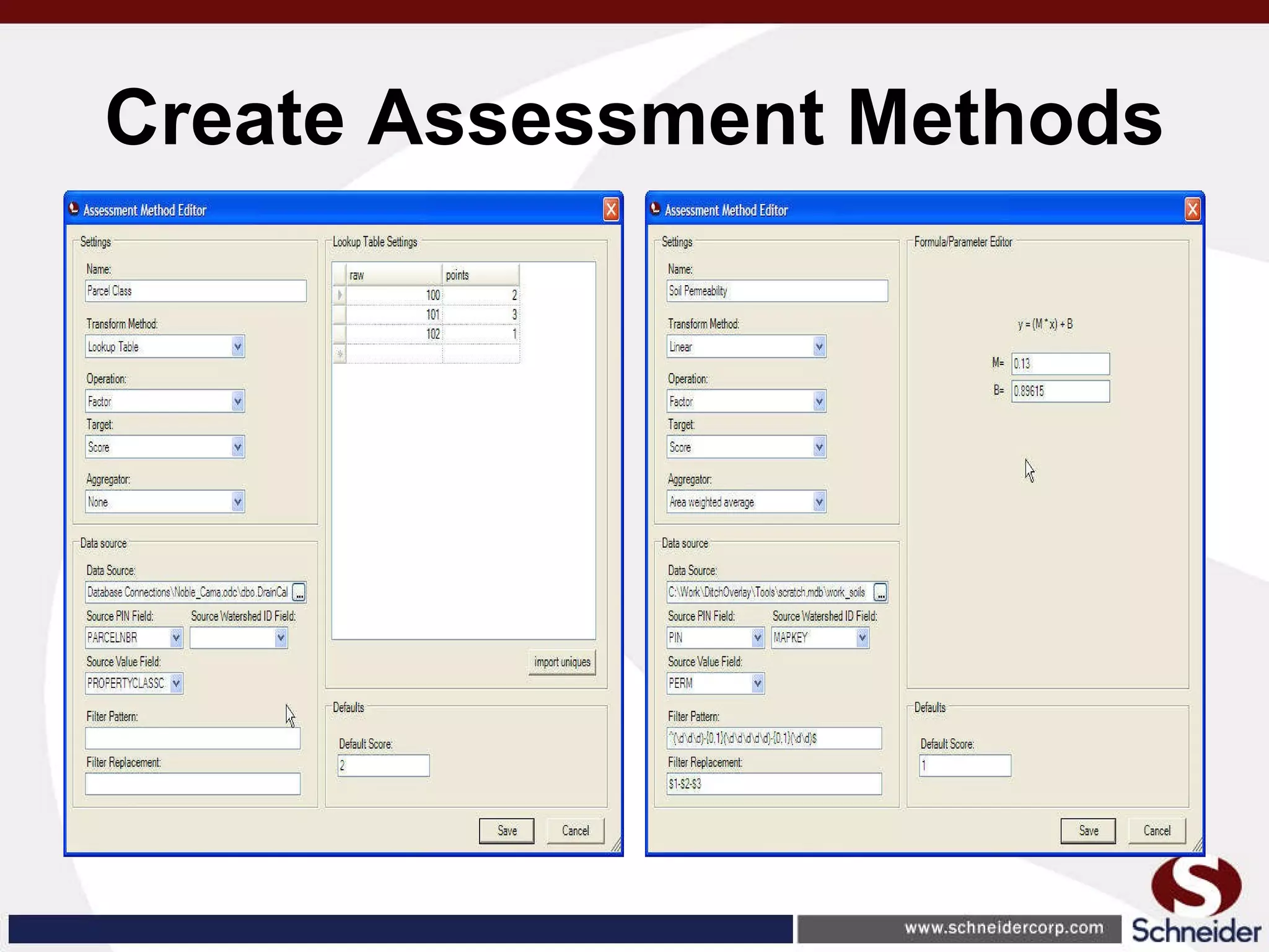
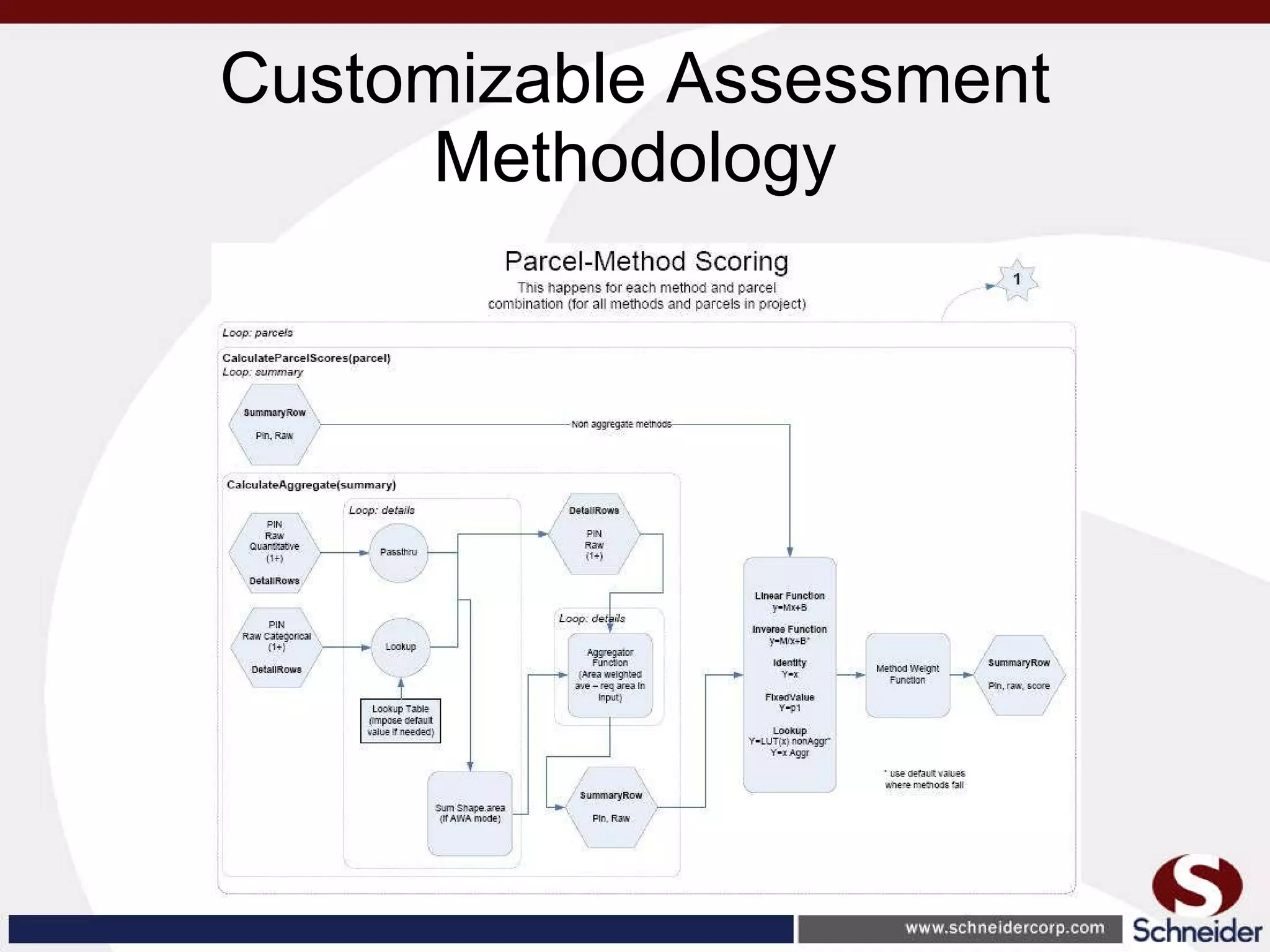
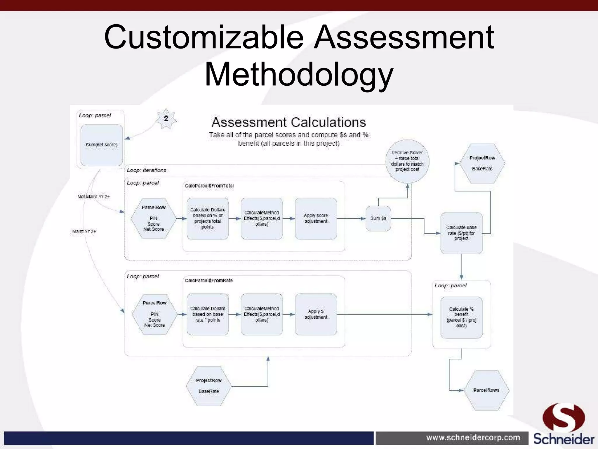
This document summarizes how GIS data and software can be used to accurately assess drainage districts and generate watersheds. Key details include generating watersheds from contour, parcel and soils data layers, accounting for sinks and peaks in elevation data, attributing computer-generated watersheds to match existing administrative boundaries, and using tools like ArcGIS and Draincalc to calculate equitable assessments for individual parcels based on watershed membership and overlay analysis. The process allows non-GIS users like local government officials to benefit from automated watershed and assessment generation to improve efficiency and accuracy over previous hand-drawn methods.


