The document summarizes a presentation on geoinformatics in hydrology and water resources. It discusses watershed analysis using GRASS GIS, including delineating watershed boundaries and factors that influence the analysis. It also covers groundwater modeling in GRASS, including defining initial conditions, parameters for modeling flow and solute transport, and a case study applying the techniques. Remote sensing and field data can be used to generate accurate modeling inputs. The presentation provides an overview of conducting watershed and groundwater analyses using open-source GIS tools in GRASS.

1. PRESENTATION BY:-
BIMAL KUMAR NAYAK
M.Sc. 2nd Year (3rd Semester)
REG. NO- 18260401004
SUB:- GEOINFORMATICS IN
HYDROLOGY & WATER RESOURCES
PAPER CODE:- MGI 511021
SUBMITTED TO:-
Prof. Arvind Chandra Pandey
HOD
Dr. Anamika Shalini Tirkey
(Assistant Professor)
DEPARTMENT OF GEOINFORMATICS
CENTRAL UNIVERSITY OF JHARKHAND

2. CONTENTS:-
• WATERSHED ANALYSIS
• INTRODUCTION TO GRASS
• GRASS GIS CAPABILITIES
• STEPS INVOLVED IN DELINEATION OF WATERSHED
• FACTOR INFLUENCING WATERSHED ANALYSIS
• APPLICATION OF WATERSHED ANALYSIS
GROUND WATER MODELLING USING GRASS
WHAT IS A MODEL?
WHAT IS THE MOTIVATION FOR MODELING?
 GROUND WATER MODELLING
 SOLUTE TRANSPORT MODELLING
CASE STUDY
REFERENCES

3. WATERSHED ANALYSIS:-
Subbasin: Larger watershed can also contain smaller
watersheds, called subbasins.
Drainage divides: The boundaries between watersheds are
termed drainage divides.
Outlets: The outlet, or pour point, is the point on the surface at
which water flows out of an area. It is the lowest point along
the boundary of a watershed.

4. STEPS INVOLVED IN DELINEATION OF WATERSHED

5. FACTOR INFLUENCING WATERSHED ANALYSIS
DEM: A 30 meter DEM likely to be too coarse to provide detailed topographic features
for geomorphic and hydrologic modeling.
Algorithm: The choice of algorithm is another important factor in watershed analysis
output.
APPLICATION OF WATERSHED ANALYSIS
 Watershed analysis is used for the management and planning of natural resources.
 To provide necessary inputs for hydrological modeling.
 Flood prediction modeling and snow melt runoff models etc.
 Watershed analysis provides catchment boundaries but also hydrological parameters
useful for management programs.

6. INTRODUCTION TO GRASS
 Geographical Resources Analysis
Support System
 GRASS was originally developed in
1985–1995 at the US Army
Construction Engineering Research
Laboratory (CERL) in Champaign,
Illinois to support land management at
military installations (Neteler and
Mitasova, 2004).
 This latest version of GRASS provides
tools for raster, vector and point
analysis as well as three dimensional
visualization and image processing.
GRASS GIS CAPABILITIES:-
Raster analysis:
Vector analysis: Digitizing (scanned raster image) with
mouse, Reclassification of vector labels, Super positioning of
vector layers
Point data analysis: Delaunay triangulation, Surface
interpolation from spot
Image processing:
Visualization: 3D surfaces with 3D query (NVIZ), Color
assignments, Histogram presentation, Map overlay, Point data
maps, Raster maps, Vector maps, Zoom / unzoom -function
Map creation: Image maps, Postscript maps, HTML maps
Geostatistics: Interface to "R" (a statistical analysis
environment), Matlab, ...
Furthermore: Erosion modelling, Landscape structure
analysis, Solution transport, Watershed analysis, Ground water
modelling.

7. WATERSHED ANALYSIS USING GRASS:-

8. THE INPUT PARAMETERS CAN BE FILLED WITH REFERENCE TO THE
FOLLOWING :-
1. Elevation raster map:- Option elevation specifies the elevation data on which entire
analysis is based. NULL (no data) cells are ignored, zero and negative values are valid
elevation data.
2. Depression raster map:- Option depression specifies the optional map of actual
depressions or sinkholes in the landscape that are large enough to slow and store surface
runoff from a storm event. All cells that are not NULL and not zero indicate depressions.
Water will flow into but not out of depressions.
3. Blocking overland surface flow:- Option blocking specifies terrain that will block
overland surface flow.
4. Threshold:- Option threshold specifies the minimum size of an exterior watershed basin
in cells, if no flow map is input, or overland flow units when a flow map is given.

9. GROUND WATER MODELLING USING GRASS
What Is a Model?
A model is a simplified representation of the complex natural world.
What is the Motivation for Ground Water Modelling ?
 How will pumping affect groundwater levels in 100 years?
 How will proposed land use change affect groundwater discharge to wetlands and streams ?
 How will water management decisions related to water diversions affect groundwater levels in the
next 50 years?
 How will climate change affect groundwater levels and groundwater discharge to surface water
bodies in temperate forests ?
 How long will it take for water levels in a lake created as a result of open pit mining to reach
equilibrium after dewatering operations cease?
 Where and when should groundwater be sampled to identify potential leakage of a clay liner beneath
a landfill ?
 How long will it take contaminants leaching into groundwater from an abandoned industrial site in
Tokyo to reach the property boundary?

10. A) GROUND WATER MODELLING

11. THE INPUT PARAMETERS REQUIRED CAN BE FILLED WITH
1. Initial Piezometric head:- Determining piezometric head is accomplished by measuring the elevation of the water
level in a well. Piezometric total head calculations in groundwater use the formula h=z+Ψ where h means total head
or height of the groundwater level above the datum, usually sea level, while z represents the elevation head
and Ψ represents the pressure head.
2. Name of the input raster map providing boundary condition status:- There are three boundary condition status
that are a) 0- inactive , b) 1- active, c) 2- dirichlet.
3. Storativity for confined or effective porosity for unconfined ground water flow :-
• Unconfined aquifer – Storativity related to effective porosity
• Confined aquifer – Storativity related to specific storage (compressibility of aquifer formation)
4. X- part and Y- part of the hydraulic conductivity tensor in (m/s)(Isotropy and anisotropy of the
environment):-

12. 5. Top suface of the aquifer:- Here we have to give the raster map
which will give us the information related to the top surface of the
aquifer.
6. Bottom surface of the aquifer:- Here we have to give the raster
map which will give us the information related to the bottom
surface of the aquifer.
7. Output raster map storing the numerical result :- Here we have
to give the location of the output raster map where we can get the
map containing the raster map.

13. SOLUTE TRANSPORT MODEL:-

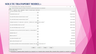
14. This numerical program calculates numerical implicit transient and steady state solute transport in porous
media in the saturated zone of an aquifer. The computation is based on raster maps and the current region
settings. All initial- and boundary-conditions must be provided as raster maps. The unit in the location must be
meters.
FORMULA FOR CALCULATING THE SOLUTE TRANSPORT
(dc/dt)*R = div ( D grad c - uc) + cs - q/nf(c - c_in)
Where,
c -- the concentration [kg/m^3]
u -- vector of mean groundwater flow velocity
dt -- the time step for transient calculation in seconds [s]
R -- the linear retardation coefficient [-]
D -- the diffusion and dispersion tensor [m^2/s]
cs -- inner concentration sources/sinks [kg/m^3]
c_in -- the solute concentration of influent water [kg/m^3]
q -- inner well sources/sinks [m^3/s]
nf -- the effective porosity [-]

15. USE OF GEOINFORMATICS AND REMOTE
SENSING :-
Remote sensing will not help in putting the every
parameters in the box which is a main drawback for
this GRASS GIS.
One should must have the knowledge about the
terrain with field observation .
Collecting the data about the well depth for
calculating the piezometric head is also very
important.
The by applying GIS using both remotely sensed data
and field survey data we are in better position to
generate the good quality map with great accuracy.

16. CASE STUDY :-
TAKEN FROM:-A new GRASS GIS
toolkit for Hortonian analysis of drainage
networks (Jaros"aw Jasiewicz a, 2 March 2011)
STUDY AREA:- Western Poland
The case study area lies in western
Poland, and covers the Koldawka Basin of
321.078 km2 in size and its
surroundings, in total 1038.427 km2. The
digital elevation model has been created
by manual digitization of hypsometric
maps with a grid resolution of 5*5 m2.
However, the DEM used in this paper had
a grid resolution of 15*15 m2.

17. METHODOLOGY:-
 Extraction of stream networks from a DEM and any accumulation
map, even those coming from any external software, according to
various user-defined criteria (r.stream.extract);
 Ordering of the extracted network and calculation of Hortonian
statistics (r.stream.order, r.stream.stats);
 Advanced modeling of basins (r.stream.basins);
 Flow path relative distance/elevation calculation (r.stream.- distance,
r.stream.slope);
 Some additional geometrical properties of ordered networks
(r.stream.segment, r.stream.channel);
 Partitioning of stream segments into near-straight-line sectors and
calculation of sector directions (r.stream.segment);
CONCLUSION:-
The new feature offered by the r.stream toolset is a new approach for
modeling and extraction of stream networks based on accumulation
map created with any flow distribution method . The possibility of
applying additional natural modifiers (e.g., geology, land cover, soil
moisture, and direct field observations) during the modeling process is
also a new quality, treating map algebra as a main tool to fine-tune
channel initiation and channel tracing. Researchers can now perform
advanced network modeling without additional programming
effort.

18.  REFERNECES:-
 https://grass.osgeo.org/documentation/general-overview/
 http://www.gisresources.com/giswatershedwatershed-analysis/
 https://www.microimages.com/documentation/TechGuides/00WatershedLP.pdf
 https://www.researchgate.net/publication/279955506_FUNDAMENTALS_OF_GROUNDWATER_MODELLING
 http://scitechconnect.elsevier.com/what-is-groundwater-modelling-why-important/
 http://external.opengis.org/twiki_public/pub/HydrologyDWG/GWIE2UC4DiscussionPage/1-s2.0-
S0098300405001585-main.pdf
 https://sciencing.com/calculate-piezometric-head-8710823.html
 https://library.wmo.int/doc_num.php?explnum_id=4835
 A new GRASS GIS toolkit for Hortonian analysis of drainage networks (Jaros"aw Jasiewicz a, 2 March 2011)