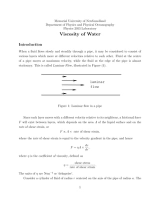
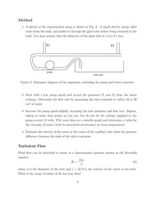
Memorial University of Newfoundland
                     Department of Physics and Physical Oceanography
                                Physics 2053 Laboratory
                               Viscosity of Water

Introduction
When a fluid flows slowly and steadily through a pipe, it may be considered to consist of
various layers which move at different velocities relative to each other. Fluid at the centre
of a pipe moves at maximum velocity, while the fluid at the edge of the pipe is almost
stationary. This is called Laminar Flow, illustrated in Figure (1).


                                                           laminar
                                                           flow


                              Figure 1: Laminar flow in a pipe


   Since each layer moves with a different velocity relative to its neighbour, a frictional force
F will exist between layers, which depends on the area A of the liquid surface and on the
rate of shear strain, or
                              F ∝ A × rate of shear strain.

where the rate of shear strain is equal to the velocity gradient in the pipe, and hence

                                                    dv
                                        F = ηA ×       ,
                                                    dr

where η is the coefficient of viscosity, defined as

                                            shear stress
                                   η=                        .
                                        rate of shear strain

The units of η are Nsm−2 or ‘dekapoise’.
  Consider a cylinder of fluid of radius r centered on the axis of the pipe of radius a. The

                                               1
surface area of the fluid cylinder (length ) is 2πr . The force exerted by the fluid outside
the cylinder on the fluid inside the cylinder is

                                                          dv
                                             F = −2πr η                                     (1)
                                                          dr

F opposes the fluid motion inside the cylinder. The ‘−’ sign is necessary because v decreases
as r increases. For steady flow, a driving force must be applied to counteract the resisting
viscous force. If P1 and P2 are the pressures at the ends of the fluid element, the net force
is given by
                                     F = (P1 − P2 )πr2 .                                 (2)

Hence we have
                                          dv
                                  − 2πr η      = (P1 − P2 )πr2                               (3)
                                          dr
and thus the velocity of a cylindrical shell (radius r) in a cylinder of radius a is given by

                                               P1 − P2 2
                                   v(r) =             (a − r2 ).                            (4)
                                                 4 η

   The total volume per unit time (i.e. the flow rate or volume flux) through the pipe is
obtained by adding up the flow due to all such shells of radius r and thickness dr. i.e.,

                              dV         a               πa4 (P1 − P2 )
                                 =           2πvr dr =                  .                   (5)
                              dt     0                        8η

This is Poiseuille’s Law (1835), and holds as long as the flow is laminar; it does not hold
for turbulent motion.


Derivation of Poiseuille’s Law by Dimensional Analysis
Poiseuille’s equation can be derived on the assumption that the volume of liquid flowing
through a pipe depends on η, a and the pressure gradient ∆p/ . Thus we have
                                                                        z
                                                                   ∆p
                             volume per second = kη x ay

where k is a constant. Use dimensional arguments to obtain values for x, y and z.


                                                   2
Method
  1. A sketch of the experimental setup is shown in Fig. 2. A small electric pump takes
     water from the tank, and pushes it through the glass tube before being returned to the
     tank. You may assume that the diameter of the glass tube is 1.2 ± 0.1 mm.


                     P1                                                 P2


                     pump
                                                          water tank


 Figure 2: Schematic diagram of the apparatus, including the pump and water reservoir.


  2. Start with a low pump speed and record the pressures P1 and P2 from the water
     columns. Determine the flow rate by measuring the time required to collect 10 or 20
     cm3 of water.

  3. Increase the pump speed slightly, recording the new pressures and flow rate. Repeat,
     taking as many data points as you can, but do not let the voltage supplied to the
     pump exceed 12 volts. Plot your data on a suitable graph and determine a value for
     the viscosity of water (with its associated uncertainty) at room temperature.

  4. Estimate the velocity of the water at the centre of the capillary tube when the pressure
     difference between the ends of the tube is greatest.


Turbulent Flow
Fluid flow can be described in terms of a dimensionless quantity known as the Reynolds
number.
                                            dvρ
                                      Re =                                        (6)
                                             η
where d is the diameter of the tube and v = Q/A is the velocity of the water in the tube.
What is the range of values of Re for your data?

                                             3
At the critical velocity, (denoted by vc ), there is a transition in the flow from laminar to
turbulent flow. For fluid flow along a cylindrical pipe, vc is given by

                                                  Rc η
                                          vc =
                                                  2aρ

where ρ is the density of the fluid and Rc is the critical Reynold’s number, which for most
fluids is approximately 2000. Estimate vc for your configuration.
   Can you observe the onset of turbulence?


                                              4

Viscosity of water

  • 1.
    Memorial University ofNewfoundland Department of Physics and Physical Oceanography Physics 2053 Laboratory Viscosity of Water Introduction When a fluid flows slowly and steadily through a pipe, it may be considered to consist of various layers which move at different velocities relative to each other. Fluid at the centre of a pipe moves at maximum velocity, while the fluid at the edge of the pipe is almost stationary. This is called Laminar Flow, illustrated in Figure (1). laminar flow Figure 1: Laminar flow in a pipe Since each layer moves with a different velocity relative to its neighbour, a frictional force F will exist between layers, which depends on the area A of the liquid surface and on the rate of shear strain, or F ∝ A × rate of shear strain. where the rate of shear strain is equal to the velocity gradient in the pipe, and hence dv F = ηA × , dr where η is the coefficient of viscosity, defined as shear stress η= . rate of shear strain The units of η are Nsm−2 or ‘dekapoise’. Consider a cylinder of fluid of radius r centered on the axis of the pipe of radius a. The 1
  • 2.
    surface area ofthe fluid cylinder (length ) is 2πr . The force exerted by the fluid outside the cylinder on the fluid inside the cylinder is dv F = −2πr η (1) dr F opposes the fluid motion inside the cylinder. The ‘−’ sign is necessary because v decreases as r increases. For steady flow, a driving force must be applied to counteract the resisting viscous force. If P1 and P2 are the pressures at the ends of the fluid element, the net force is given by F = (P1 − P2 )πr2 . (2) Hence we have dv − 2πr η = (P1 − P2 )πr2 (3) dr and thus the velocity of a cylindrical shell (radius r) in a cylinder of radius a is given by P1 − P2 2 v(r) = (a − r2 ). (4) 4 η The total volume per unit time (i.e. the flow rate or volume flux) through the pipe is obtained by adding up the flow due to all such shells of radius r and thickness dr. i.e., dV a πa4 (P1 − P2 ) = 2πvr dr = . (5) dt 0 8η This is Poiseuille’s Law (1835), and holds as long as the flow is laminar; it does not hold for turbulent motion. Derivation of Poiseuille’s Law by Dimensional Analysis Poiseuille’s equation can be derived on the assumption that the volume of liquid flowing through a pipe depends on η, a and the pressure gradient ∆p/ . Thus we have z ∆p volume per second = kη x ay where k is a constant. Use dimensional arguments to obtain values for x, y and z. 2
  • 3.
    Method 1.A sketch of the experimental setup is shown in Fig. 2. A small electric pump takes water from the tank, and pushes it through the glass tube before being returned to the tank. You may assume that the diameter of the glass tube is 1.2 ± 0.1 mm. P1 P2 pump water tank Figure 2: Schematic diagram of the apparatus, including the pump and water reservoir. 2. Start with a low pump speed and record the pressures P1 and P2 from the water columns. Determine the flow rate by measuring the time required to collect 10 or 20 cm3 of water. 3. Increase the pump speed slightly, recording the new pressures and flow rate. Repeat, taking as many data points as you can, but do not let the voltage supplied to the pump exceed 12 volts. Plot your data on a suitable graph and determine a value for the viscosity of water (with its associated uncertainty) at room temperature. 4. Estimate the velocity of the water at the centre of the capillary tube when the pressure difference between the ends of the tube is greatest. Turbulent Flow Fluid flow can be described in terms of a dimensionless quantity known as the Reynolds number. dvρ Re = (6) η where d is the diameter of the tube and v = Q/A is the velocity of the water in the tube. What is the range of values of Re for your data? 3
  • 4.
    At the criticalvelocity, (denoted by vc ), there is a transition in the flow from laminar to turbulent flow. For fluid flow along a cylindrical pipe, vc is given by Rc η vc = 2aρ where ρ is the density of the fluid and Rc is the critical Reynold’s number, which for most fluids is approximately 2000. Estimate vc for your configuration. Can you observe the onset of turbulence? 4