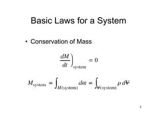
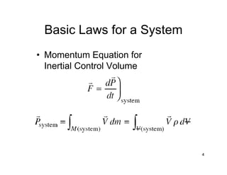
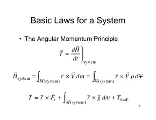
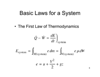
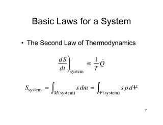
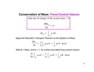
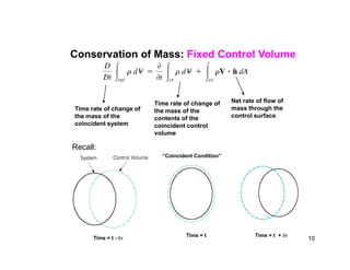
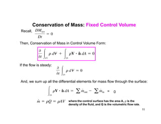
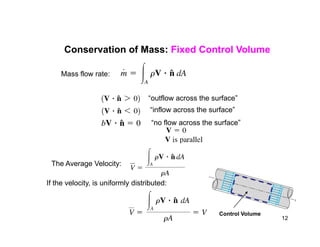
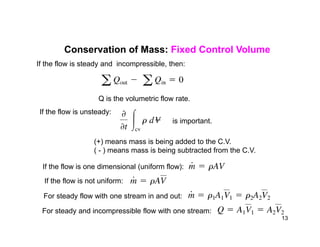
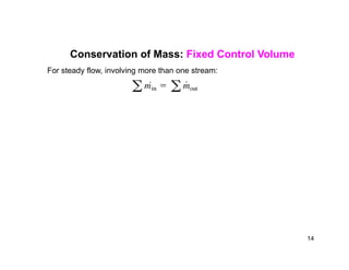
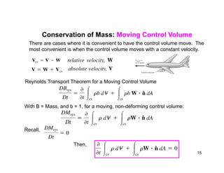
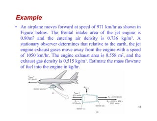
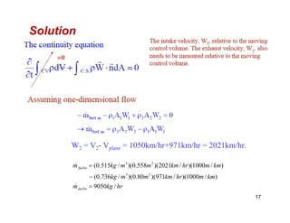
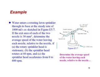
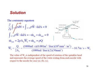
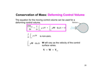
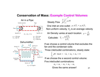
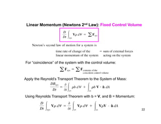
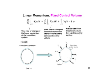
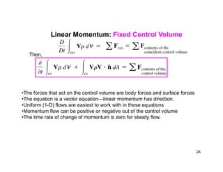
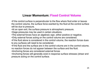
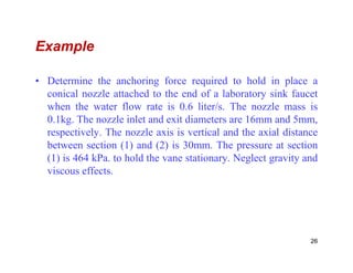
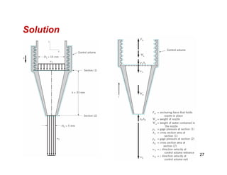
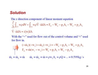
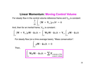
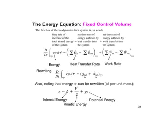
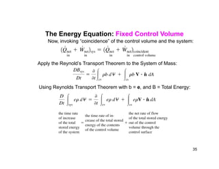
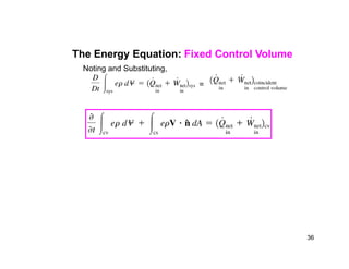
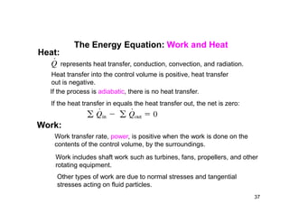
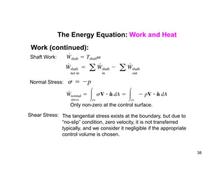
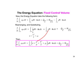
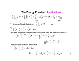
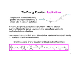
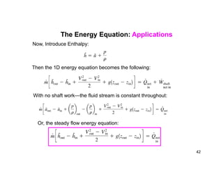
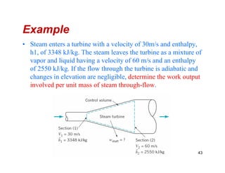
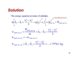
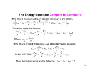
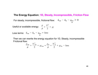
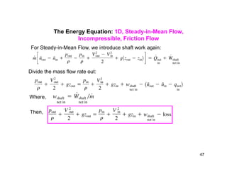
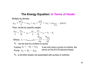
The document discusses control volume analysis and the conservation laws applied to control volumes, including: - Conservation of mass for fixed, moving, and deforming control volumes - Linear momentum (Newton's second law) for fixed control volumes - The energy equation for fixed control volumes, including work, heat transfer, and applications to steady, incompressible flow - An example problem calculating the work output of steam passing through a turbine using the energy equation

1. Lecture 5: Control Volume Analysis
1

2. Outline
• Introduction
• Basic Laws for a System
• Conservation of Mass
• Linear Momentum• Linear Momentum
• Energy Equation
• Examples
2

3. Basic Laws for a System
• Conservation of Mass
3

4. Basic Laws for a System
• Momentum Equation for
Inertial Control Volume
4

5. Basic Laws for a System
• The Angular Momentum Principle
5

6. Basic Laws for a System
• The First Law of Thermodynamics
6

7. Basic Laws for a System
• The Second Law of Thermodynamics
7

8. Control Volume Analysis: Introduction
• Practical problems involve finite regions
• We call these regions control volumes
• Physical laws govern these regions
• We Apply Conservation Laws• We Apply Conservation Laws
• We look at Mass, Momentum, and Energy
of the Region
8

9. Conservation of Mass: Fixed Control Volume
Apply the Reynold’s Transport Theorem to the System of Mass:
With B = Mass, and b = 1, for a fixed non-deforming control volume:
9

10. Conservation of Mass: Fixed Control Volume
Time rate of change of
the mass of the
coincident system
Time rate of change of
the mass of the
contents of the
coincident control
volume
Net rate of flow of
mass through the
control surface
volume
Recall:
“Coincident Condition”
Time = t
Time = t - 
Time = t + 
10

11. Conservation of Mass: Fixed Control Volume
Recall,
Then, Conservation of Mass in Control Volume Form:
If the flow is steady:
And, we sum up all the differential elements for mass flow through the surface:
= 0
where the control surface has the area A,  is the
density of the fluid, and Q is the volumetric flow rate.
11

12. Conservation of Mass: Fixed Control Volume
“outflow across the surface”
“inflow across the surface”
“no flow across the surface”
Mass flow rate:
“no flow across the surface”
The Average Velocity:
If the velocity, is uniformly distributed:
Control Volume
12

13. Conservation of Mass: Fixed Control Volume
If the flow is steady and incompressible, then:
Q is the volumetric flow rate.
If the flow is unsteady:
is important.is important.
(+) means mass is being added to the C.V.
( - ) means mass is being subtracted from the C.V.
If the flow is one dimensional (uniform flow):
If the flow is not uniform:
For steady flow with one stream in and out:
For steady and incompressible flow with one stream:
13

14. Conservation of Mass: Fixed Control Volume
For steady flow, involving more than one stream:
14

15. There are cases where it is convenient to have the control volume move. The
most convenient is when the control volume moves with a constant velocity.
Conservation of Mass: Moving Control Volume
Reynolds Transport Theorem for a Moving Control Volume
With B = Mass, and b = 1, for a moving, non-deforming control volume:
Recall,
Then,
15

16. Example
• An airplane moves forward at speed of 971 km/hr as shown in
Figure below. The frontal intake area of the jet engine is
0.80m2 and the entering air density is 0.736 kg/m3. A
stationary observer determines that relative to the earth, the jet
engine exhaust gases move away from the engine with a speed
of 1050 km/hr. The engine exhaust area is 0.558 m2, and the
exhaust gas density is 0.515 kg/m3. Estimate the mass flowrateexhaust gas density is 0.515 kg/m3. Estimate the mass flowrate
of fuel into the engine in kg/hr.
16

17. Solution
hrkgm
kmmhrkmmmkg
kmmhrkmmmkgm
fuelin
fuelin
/9050
)/1000)(/971)(80.0)(/736.0(
)/1000)(/2021)(558.0)(/515.0(
23
23





W2 = V2- Vplane = 1050km/hr+971km/hr = 2021km/hr.
17

18. Example
18

19. Solution
19

20. Conservation of Mass: Deforming Control Volume
The equation for the moving control volume can be used for a
deforming control volume.
is non-zero.is non-zero.
W will vary as the velocity of the control
surface varies.
20

21. Conservation of Mass: Example Control Volumes
One inlet an one outlet:
Air in a Pipe:
Steady Flow
Non-uniform velocity, V2 is an average velocity
Air Density varies at each location
Calculate:Calculate:
If we choose a control volume that excludes the
fan and the condenser coils:
Dehumidifier:
Three inlet/outlet combinations, steady state:
If we choose the a second control volume:
Gives the same answer!
Five inlet/outlet combinations:
21

22. Linear Momentum (Newtons 2nd Law): Fixed Control Volume
For “coincidence” of the system with the control volume:For “coincidence” of the system with the control volume:
Using Reynolds Transport Theorem with b = V, and B = Momentum:
Apply the Reynold’s Transport Theorem to the System of Mass:
22

23. Linear Momentum: Fixed Control Volume
Time rate of change of
the linear momentum
of the coincident
system
Time rate of change of
the linear momentum
of the contents of the
coincident control
volume
Net rate of flow of
linear momentum
through the control
surface
volume
Recall:
“Coincident Condition”
Time = t 23

24. Linear Momentum: Fixed Control Volume
Then,
•The forces that act on the control volume are body forces and surface forces
•The equation is a vector equation—linear momentum has direction.
•Uniform (1-D) flows are easiest to work with in these equations
•Momentum flow can be positive or negative out of the control volume
•The time rate of change of momentum is zero for steady flow.
24

25. Linear Momentum: Fixed Control Volume
•If the control surface is perpendicular to the flow where fluid enter or leaves
the control volume, the surface force exerted by the fluid at the control surface
will be due to pressure.
•At an open exit, the surface pressure is atmospheric pressure.
•Gage pressures may be used in certain situations.
•The external forces have an algebraic sign, either positive or negative.
•Only external forces acting on the control volume are considered.•Only external forces acting on the control volume are considered.
•If the fluid alone is considered in the control volume, the reaction forces dues
to any surfaces will need to be considered.
•If the fluid and the surface are in the control volume are in the control volume,
no reaction forces do not appear between the surface and the fluid.
•Anchoring forces are considered external forces
•Anchoring forces will generally exist in response surface stresses (shear and
pressure acting on the control surface.
25

26. Example
• Determine the anchoring force required to hold in place a
conical nozzle attached to the end of a laboratory sink faucet
when the water flow rate is 0.6 liter/s. The nozzle mass is
0.1kg. The nozzle inlet and exit diameters are 16mm and 5mm,
respectively. The nozzle axis is vertical and the axial distancerespectively. The nozzle axis is vertical and the axial distance
between section (1) and (2) is 30mm. The pressure at section
(1) is 464 kPa. to hold the vane stationary. Neglect gravity and
viscous effects.
26

27. Solution
27

28. Solution
28

29. Solution
29

30. Example
• A static thrust as sketched in Figure below is to be designed
for testing a jet engine. The following conditions are known
for a typical test: Intake air velocity = 200 m/s; exhaust gas
velocity=500 m/s; intake cross-section area = 1m2; intake
static pressure = -22.5 kPa=78.5 kPa (abs); intake static
temperature = 268K; exhaust static pressure = 0 kPa=101 kPatemperature = 268K; exhaust static pressure = 0 kPa=101 kPa
(abs). Estimate the normal trust for which to design.
30

31. Solution
31

32. Linear Momentum: Moving Control Volume
Reynolds Transport Theorem for a Moving Control Volume
With B = Momentum, and b = V, for a fixed non-deforming control volume:
Then, substituting the above equation:
Substitute for V:
32

33. Linear Momentum: Moving Control Volume
For steady flow in the control volume reference frame and VCV is constant:
And, then for an inertial frame, VCV is constant :
For steady flow (on a time average basis), “Mass conservation”:
Then,
33

34. The Energy Equation: Fixed Control Volume
Heat Transfer Rate Work RateEnergy
Rewriting,
Also, noting that energy, e, can be rewritten (all per unit mass):
Internal Energy
Kinetic Energy
Potential Energy
34

35. The Energy Equation: Fixed Control Volume
Now, invoking “coincidence” of the control volume and the system:
Using Reynolds Transport Theorem with b = e, and B = Total Energy:
Apply the Reynold’s Transport Theorem to the System of Mass:
Using Reynolds Transport Theorem with b = e, and B = Total Energy:
35

36. The Energy Equation: Fixed Control Volume
Noting and Substituting,
=
36

37. The Energy Equation: Work and Heat
represents heat transfer, conduction, convection, and radiation.
Heat transfer into the control volume is positive, heat transfer
out is negative.
If the process is adiabatic, there is no heat transfer.
If the heat transfer in equals the heat transfer out, the net is zero:
Heat:
Work:
Work transfer rate, power, is positive when the work is done on the
contents of the control volume, by the surroundings.
Work includes shaft work such as turbines, fans, propellers, and other
rotating equipment.
Other types of work are due to normal stresses and tangential
stresses acting on fluid particles.
37

38. The Energy Equation: Work and Heat
Work (continued):
Shaft Work:
Normal Stress:
Shear Stress:
Only non-zero at the control surface.
The tangential stress exists at the boundary, but due to
“no-slip” condition, zero velocity, it is not transferred
typically, and we consider it negligible if the appropriate
control volume is chosen.
38

39. The Energy Equation: Fixed Control Volume
Now, the Energy Equation take the following form:
+ =
Rearranging, and Substituting,
Then,
39

40. The Energy Equation: Applications
(1) (2) (3)
(1) Assume Steady Sate then, = 0
(2)
Assume properties are uniformly distributed over the flow cross-section,
Assume one inlet and one outlet:
40

41. The Energy Equation: Applications
However, the previous assumption of uniform 1D flow is often an
oversimplification for control volumes, but its ease of use justifies it’s
application to these situations.
The previous assumption is fairly
good for a fluid particle following a
stream tube in a steady state flow.
application to these situations.
Now, we can introduce shaft work. We note that shaft work is unsteady locally,
but its effects downstream are steady.
One Dimensional Energy Equation for Steady-in-the-Mean Flow:
41

42. The Energy Equation: Applications
Now, Introduce Enthalpy:
Then the 1D energy equation becomes the following:
With no shaft work—the fluid stream is constant throughout:
Or, the steady flow energy equation:
42

43. Example
• Steam enters a turbine with a velocity of 30m/s and enthalpy,
h1, of 3348 kJ/kg. The steam leaves the turbine as a mixture of
vapor and liquid having a velocity of 60 m/s and an enthalpy
of 2550 kJ/kg. If the flow through the turbine is adiabatic and
changes in elevation are negligible, determine the work output
involved per unit mass of steam through-flow.involved per unit mass of steam through-flow.
43

44. Solution
44

45. The Energy Equation: Compare to Bernoulli’s
If the flow is incompressible, in addition to being 1D and steady,
Divide the mass flow rate out:
Where,
If the flow is inviscid (frictionless), we obtain Bernoulli’s equation:
or, per unit mass,
Thus, the friction terms are the following:
45

46. The Energy Equation: 1D, Steady, Incompressible, Friction Flow
For steady, incompressible, frictional flow:
Useful or available energy:
Loss terms:
Then we can rewrite the energy equation for 1D, Steady, incompressibleThen we can rewrite the energy equation for 1D, Steady, incompressible
Frictional flow:
46

47. The Energy Equation: 1D, Steady-in-Mean Flow,
Incompressible, Friction Flow
For Steady-in-Mean Flow, we introduce shaft work again:
Divide the mass flow rate out:
Where,
Then,
47

48. The Energy Equation: In Terms of Heads
Multiply by density:
Then, divide by specific weight:
Where,
Turbine:
Pump:
is all other losses not associated with pumps or turbines
can be due to a turbine or pump
If we only have a pump or turbine, the
terms on the R.H.S become these.
48

49. Example
• An axial-flow ventilating fan driven by a motor that delivers
0.4 kW of power to the fan blades produces a 0.6-m-diameter
axial stream of air having a speed of 12 m/s. The flow
upstream of the fan involves negligible speed. Determine how
much of the work to the air actually produces a useful effects,
that is, a rise in available energy and estimate the fluidthat is, a rise in available energy and estimate the fluid
mechanical efficiency of this fan.
49

50. Solution
50
752.0
8.95
72
