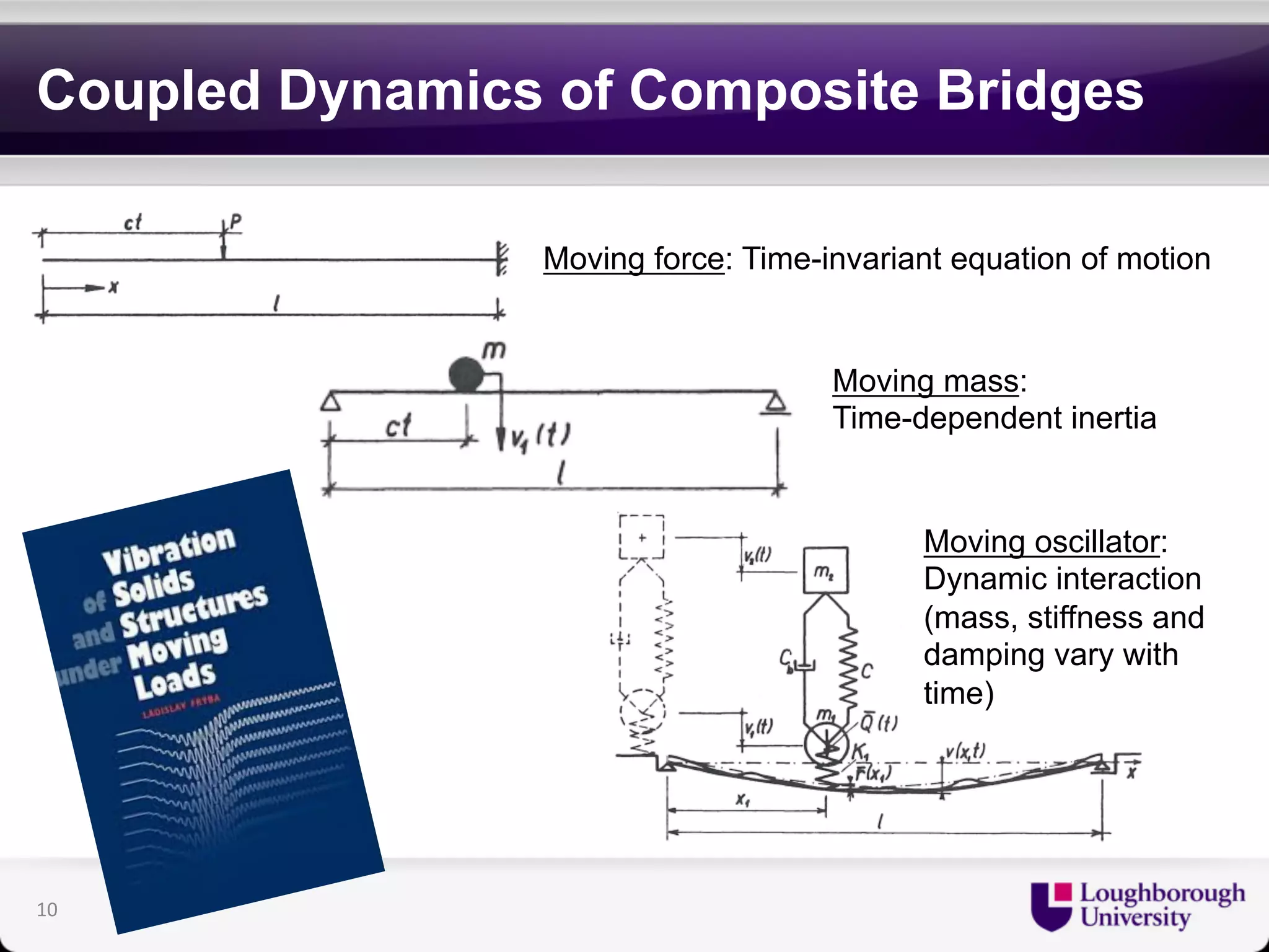
Download as PDF, PPTX

![Coupled Dynamics of Composite Bridges
! Cascade'equations'of'motion:'
⎪⎪⎨⎪
⎧ ⎧ ∂ 2 ⎫ ∂ 2 ⎧ ∂ 2 ⎫ ∂ 4 ⎧ ∂ 2
⎫ ⎪ ⎨ − + ∂ ⎬ ∂ ⎨ − ⎬ + = ∂ ∂ ⎨ − ∂ ⎬ ⎩ ⎭ ⎩ ⎭ ⎩ ⎭ ⎪∂ ⎛ ∂ ∂ ∂ ⎞ = ⎜ + − − ⎩⎪ ∂ ⎝ ∂ ∂ ∂ ⎟ ⎠
A v z t EI v z t R z t f z t
1 1 ( , ) 1 1 ( , ) ( , ) 1 1 ( , ) ,
b 2 2 2 b( ) 2 2 4 b 2 2 b
z t z z z
b b b
w z t f z t K d v z t A v z t EI v z t
z rEA z t z
( , ) 1 ( , ) ( , ) ( , ) ( , ) ;
! where:'
b b
f A A Agρ = ρ +ρ +
[ ]
[ ] [ ]
[ ]
(s)
b
b c c s s
EI E I E I
b(0) c c s s
EI EI E E A A d
c s c s 2
b( ) b(0) b
∞ E A E A
c c s s
= +
= +
+
Composite$beam$transverse$deflections$
2 2 4
[ ] [ ]
[ ]
[ ]
[ ]
[ ] [ ]
[ ]
2
2 i b
b
b(0)
b(0)
b( )
2
2 2 b(0) i b
b b
b( ) b(0)
b( )
b( )
1
;
1
K d
EI
EI
EI
EI K d
EI EI
EI
EI
α
β α
∞
∞
∞
∞
=
⎛ ⎞
⎜ − ⎟
⎜⎝ ⎟⎠
= =
⎛ ⎞
⎜ − ⎟
⎜⎝ ⎟⎠
Non$Composite$
Fully$Composite$
Concrete$slab$axial$displacements$
[ ] [ ]
[ ] [ ]
c 2
2 b i b 2 b b 2 b b(0) 4 b
b b c c
ρ
β α β
ρ
β
∞
13
Vibration of the beam: Governing equation](https://image.slidesharecdn.com/leedspresentationnovember2014-141128175038-conversion-gate02/75/Using-blurred-images-to-assess-damage-in-bridge-structures-13-2048.jpg)
![Coupled Dynamics of Composite Bridges
! Modal&equations&of&motion:&
2 ⋅qb (t) = Jb ⋅Qb (t)
qb (t) + Ξb ⋅ qb (t) +Ωb
⎧ ⎫
( ) ( ( )) ( ) ( ( )) 1 ( ( ))
Q Σ φ φ
= ⎨ − ′′ ⎬
t χ z t f t z t z t
2 1 2
J = ⎡⎣I + Δm ⎤⎦ − b
1
b n bi
Ω J Ω k
b b b() bi
Ξ Ω
b b b 2ζ
−
∞ = ⎡⎣ ⋅ ⎡⎣ + Δ ⎤⎦⎤⎦
=
b( ) b( ,1) b( ,2) b( , b ) Diag n ω ω ω ∞ ∞ ∞ ∞ Ω = ⎡⎣ L ⎤⎦
[ ]
[ ]
2
⎛ ⎞ ∞
=⎜ ⎟
⎝ ⎠
b( )
b( )
b b
j
j EI
L A
ω π
ρ
1
⎡ ⎤
π
m N
Δ = bi 2 ⎢ b
⎥
[EI]
L
β
⎣ ⎦
b b
∞ ⎡ ⎤
k N
Δ = ⎢ ⎥
[ ]
2
6
b( )
π
bi 2 b
A L
α ρ
⎣ ⎦
b b b
[ ] b b N = Diag 1 2 L n
v
b b v( ) v( ) b v( ) 2 b v( )
1 b
n
i i i i
i
= β
⎩ ⎭
15
Vibration of the beam: Modal analysis](https://image.slidesharecdn.com/leedspresentationnovember2014-141128175038-conversion-gate02/75/Using-blurred-images-to-assess-damage-in-bridge-structures-15-2048.jpg)
![Coupled Dynamics of Composite Bridges
! Finally'the'two'matrix'equations'are'rewritten'in'an'enlarged'
modal'space:'
q(t) + c0 + Δc(t) ⎡⎣
⎤⎦
⋅ q(t) + k0 + Δk(t) ⎡⎣
⎤⎦
⋅q(t) = Q(t)
O
⎡ = ⎢ n v ×
n
⎤
b
⎥
⎢⎣ b v
⎥⎦
O C
⎡ − ⋅ ⎤
v v
v
c 0
O
b
v vb
bv v b
( )
( )
( ) ( )
n n
n n t
t
t t
×
×
c
Δ = ⎢⎣− ⎢ C ⋅ Δ C
⎥ ⎥⎦
Ξ
Ξ
μ
μ
T (t) Q b
{ T (t) }T
v b
b v
O
O
[ ]
O K L
v v
2
v
0 2
b
( ) ( )
v vb vb
k
μ
bv v b
( )
( ) ( )
n n
n n
n n t t
t
t t
×
×
×
⎡ Ω ⎤
= ⎢ ⎥
⎢ Ω ⎥ ⎣ ⎦
⎡ − ⋅ + ⎤
Δ =⎢ ⎥
⎢⎣− ⋅ Δ ⎥⎦
k
K μ
K
{ T T }T
v b q(t) = q (t) q (t) Q(t) = Q v
“Small”'modifications'
20
Coupled vibration: Proposed model](https://image.slidesharecdn.com/leedspresentationnovember2014-141128175038-conversion-gate02/75/Using-blurred-images-to-assess-damage-in-bridge-structures-20-2048.jpg)
![Coupled Dynamics of Composite Bridges
! Single'step+(unconditionally+stable)+numerical+integration:+
{[ ] [ ] [ ] } 0 01 01 02 x(t + Δt) = E(t) ⋅ Θ + Γ ⋅ΔD(t) ⋅ x(t) + Γ ⋅V ⋅Q(t) + Γ ⋅V ⋅Q(t + Δt)
! Reference+transition+matrix+without+dynamic+interaction:+
L I D
Γ Θ
! Dynamic+modification+matrix:+
= ⎡⎣ Θ
− n +
n
⎤⎦ ⋅
−
= ⎡ − ⎤ ⎢⎣ Δ ⎥⎦
⋅ = ⎡ ⎤ ⎢⎣− Δ ⎥⎦
⋅ 0 0 2( ) 0
v b
1
−
L D
01 0 0 0
1
L I D
n n
t
−
+
02 0 2( ) 0
v b
1
1
1
t
2( ) 02 ( ) ( ) n n t t t −
v b
1
+ E = ⎡⎣Ι − Γ ⋅ΔD + Δ ⎤⎦
Γ
[ ] 0 0 Θ = exp D Δt
21
Coupled vibration: Proposed numerical scheme](https://image.slidesharecdn.com/leedspresentationnovember2014-141128175038-conversion-gate02/75/Using-blurred-images-to-assess-damage-in-bridge-structures-21-2048.jpg)


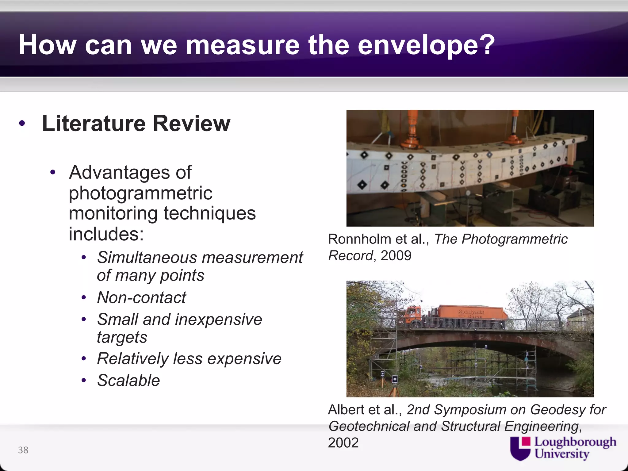

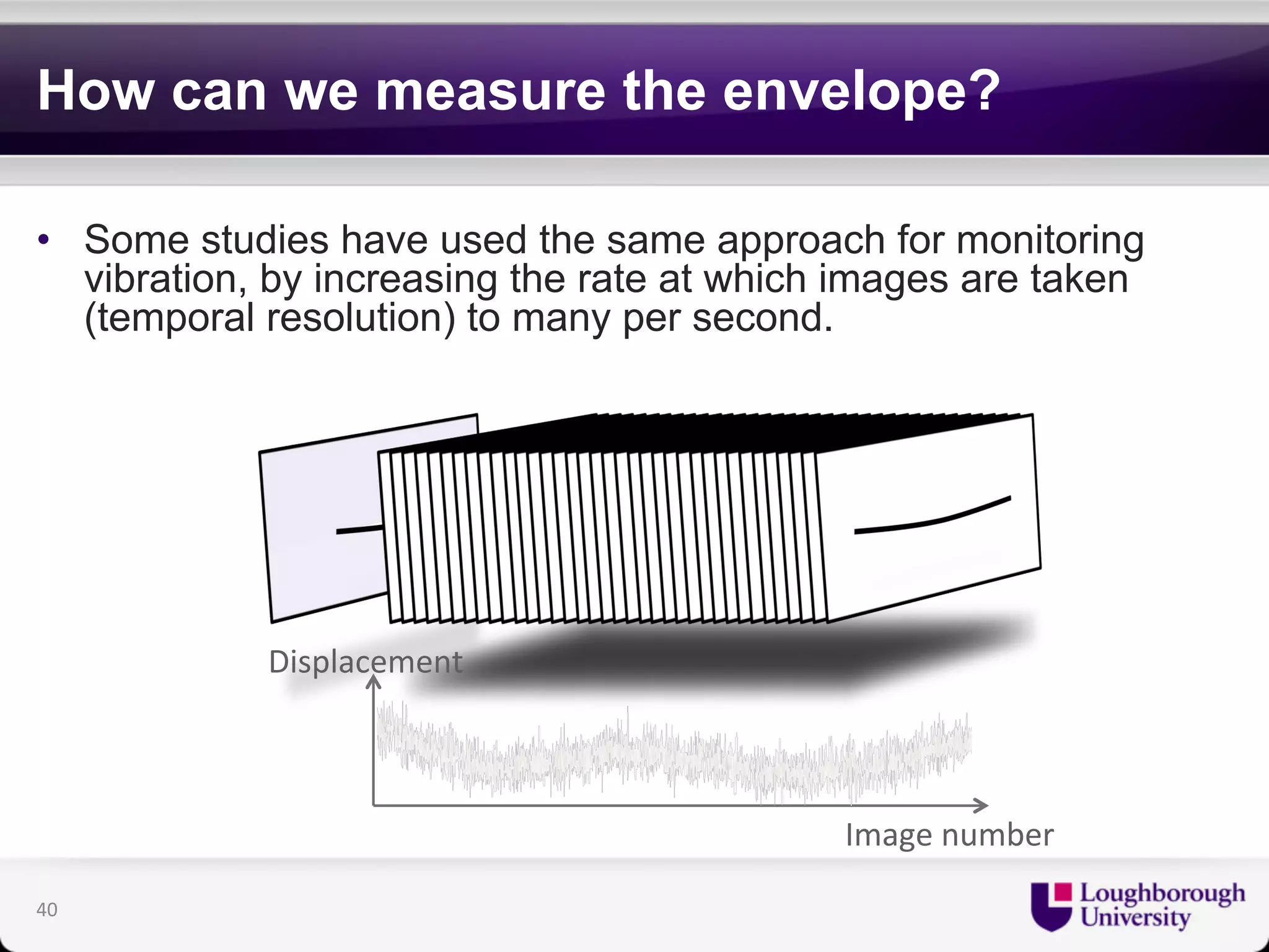
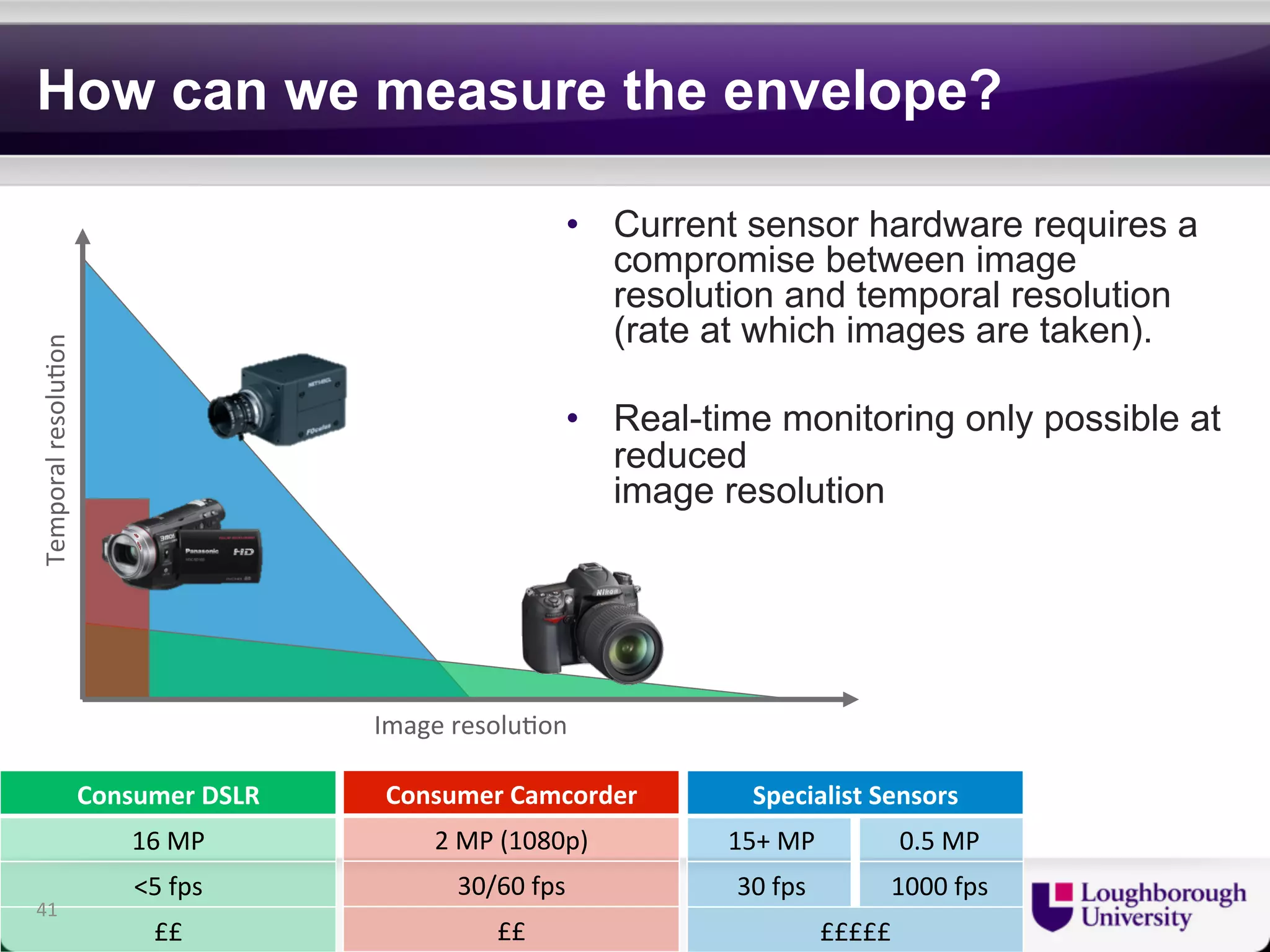


The document discusses research on the coupled dynamics of composite bridges, focusing on the effects of shear connections between steel and concrete components on bridge performance. It covers various analytical, numerical, and experimental studies addressing damage sensitivity and measurement methods. Key topics include dynamic interactions under moving forces, state-space representations of motion, and implications for structural health monitoring.


