This document introduces concepts related to dynamic response and the time domain analysis of systems. It discusses important input signals like step, ramp, and impulse functions. The response of a linear time-invariant system to various inputs is examined. The Laplace transform is introduced as a tool to simplify the analysis by converting differential equations into algebraic equations. Properties of the Laplace transform like superposition, time delay, and convolution are covered. Methods for taking the inverse Laplace transform are also presented.
![ECE4510/ECE5510, DYNAMIC RESPONSE 3–3
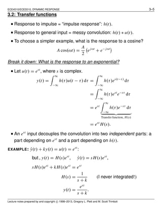
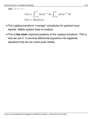
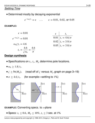
Time response of a linear time invariant system
■ Let y(t) be the output of an LTI system with input x(t).
y(t) = T[x(t)]
= T
∞
−∞
x(τ)δ(t − τ) dτ (sifting)
=
∞
−∞
x(τ)T[δ(t − τ)] dτ. (linear)
Let h(t, τ) = T[δ(t − τ)]
=
∞
−∞
x(τ)h(t, τ) dτ
If the system is time invariant, h(t, τ) = h(t − τ)
=
∞
−∞
x(τ)h(t − τ) dτ (time invariant)
△
= x(t) ∗ h(t).
■ The output of an LTI system is equal to the convolution of its impulse
response with the input.
■ This makes life EASY (TRUST me!)
EXAMPLE: Finding an impulse response:
■ Consider a first-order system, ˙y(t) + ky(t) = u(t).
■ Let y(0−
) = 0, u(t) = δ(t).
■ For positive time we have ˙y(t) + ky(t) = 0. Recall from your
differential-equation math course: y(t) = Aest
, solve for A, s.
˙y(t) = Asest
Lecture notes prepared by and copyright c⃝ 1998–2013, Gregory L. Plett and M. Scott Trimboli](https://image.slidesharecdn.com/ece4510-notes03-170714151943/85/Ece4510-notes03-3-320.jpg)
![ECE4510/ECE5510, DYNAMIC RESPONSE 3–12
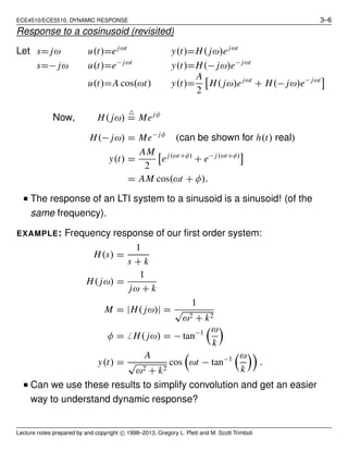
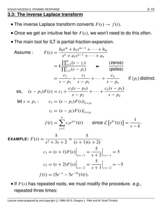
■ Lastly, we find C,
C =
s + 2
(s + 1)2
s=−3
= −
1
4
.
■ Therefore, the inverse Laplace transform we are looking for is
h(t) =
1
2
te−t
+
1
4
e−t
−
1
4
e−3t
1(t).
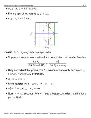
EXAMPLE: Find ILT of
s + 3
(s + 1)(s + 2)2
.
■ ans: f (t) = (2e−t
− 2e−2t
− te−2t
from repeated root.
)1(t).
■ Note that this is quite tedious, but MATLAB can help.
■ Try MATLAB with two examples; first, F(s) =
5
s2 + 3s + 2
.
Example 1. Example 2.
>> Fnum = [0 0 5]; >> Fnum = [0 0 1 3];
>> Fden = [1 3 2]; >> Fden = conv([1 1],conv([1 2],[1 2]));
[r,p,k] = residue(Fnum,Fden); [r,p,k] = residue(Fnum,Fden);
r = -5 r = -2
5 -1
p = -2 2
-1 p = -2
k = [] -2
-1
k = []
■ When you use “residue” and get repeated roots, BE SURE to type
“help residue” to correctly interpret the result.
Lecture notes prepared by and copyright c⃝ 1998–2013, Gregory L. Plett and M. Scott Trimboli](https://image.slidesharecdn.com/ece4510-notes03-170714151943/85/Ece4510-notes03-12-320.jpg)
![ECE4510/ECE5510, DYNAMIC RESPONSE 3–13
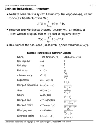
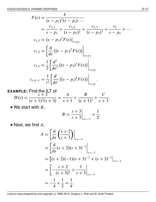
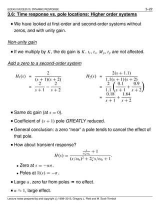
Using the Laplace transform to solve problems
■ We can use the Laplace transform to solve both homogeneous and
forced differential equations.
EXAMPLE: ¨y(t) + y(t) = 0, y(0−
) = α, ˙y(0−
) = β.
s2
Y(s) − αs − β + Y(s) = 0
Y(s)(s2
+ 1) = αs + β
Y(s) =
αs + β
s2 + 1
=
αs
s2 + 1
+
β
s2 + 1
.
From tables, y(t) = [α cos(t) + β sin(t)]1(t).
■ If initial conditions are zero, things are very simple.
EXAMPLE:
¨y(t)+5 ˙y(t)+4y(t) = u(t), y(0−
) = 0, ˙y(0−
) = 0, u(t) = 2e−2t
1(t).
s2
Y(s) + 5sY(s) + 4Y(s) =
2
s + 2
Y(s) =
2
(s + 2)(s + 1)(s + 4)
=
−1
s + 2
+
2/3
s + 1
+
1/3
s + 4
.
From tables, y(t) = −e−2t
+
2
3
e−t
+
1
3
e−4t
1(t).
Lecture notes prepared by and copyright c⃝ 1998–2013, Gregory L. Plett and M. Scott Trimboli](https://image.slidesharecdn.com/ece4510-notes03-170714151943/85/Ece4510-notes03-13-320.jpg)
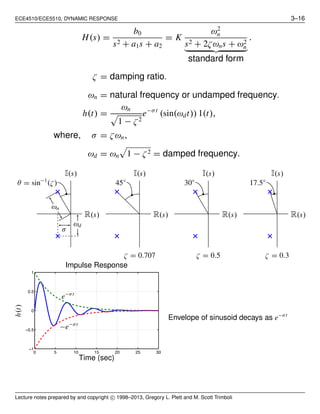
![ECE4510/ECE5510, DYNAMIC RESPONSE 3–15
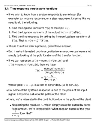
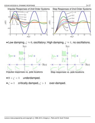
• That is, the poles qualitatively determine the behavior of the
system; zeros (equivalently, residues) quantify this relationship.
■ Note that the poles pk may be real, or they may occur in
complex-conjugate pairs.
■ So, in the next sections, we look at the time responses of real poles
and of complex-conjugate poles.
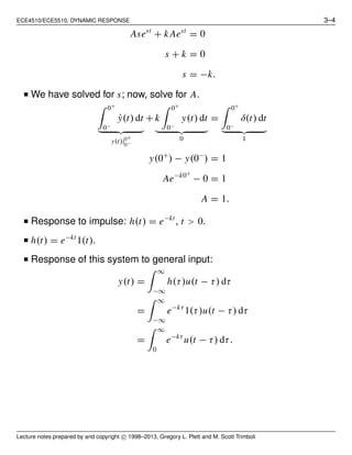
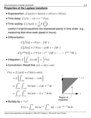
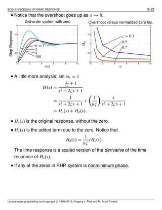
Time response due to a real pole
■ Consider a transfer function having a single real pole:
H(s) =
1
s + σ
➠ h(t) = e−σt
1(t).
■ If σ > 0, pole is at s < 0, STABLE i.e., impulse response decays, and
any bounded input produces bounded output.
■ If σ < 0, pole is at s > 0, UNSTABLE.
■ σ is “time constant” factor: τ = 1/σ.
0 1 2 3 4 5
0
0.2
0.4
0.6
0.8
1
impulse([0 1],[1 1]);
Time (sec × τ)
t = τ
←−
1
e
e−σt
h(t)
0 1 2 3 4 5
0
0.2
0.4
0.6
0.8
1
step([0 1],[1 1]);
Time (sec × τ)
t = τ
y(t)×K
K(1 − e−t/τ
)
System response. K = dc gain
Response to initial condition
−→ 0.
Time response due to complex-conjugate poles
■ Now, consider a second-order transfer function having
complex-conjugate poles
Lecture notes prepared by and copyright c⃝ 1998–2013, Gregory L. Plett and M. Scott Trimboli](https://image.slidesharecdn.com/ece4510-notes03-170714151943/85/Ece4510-notes03-15-320.jpg)
![ECE4510/ECE5510, DYNAMIC RESPONSE 3–24
0 2 4 6 8 10
−0.5
0
0.5
1
1.5
2
H(s)
Ho(s)
Hd(s)
Time (sec)
y(t)
2nd-order min-phase step resp.
0 2 4 6 8 10
−1.5
−1
−0.5
0
0.5
1
1.5
Ho(s)
H(s)
Hd(s)
Time (sec)
y(t)
2nd-order nonmin-phase step resp.
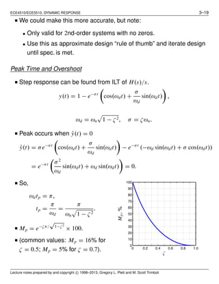
Add a pole to a second order system
H(s) =
1
s
αζωn
+ 1 [(s/ωn)2 + 2ζs/ωn + 1]
.
■ Original poles at R(s) = −σ = −ζωn.
■ New pole at s = −αζωn.
■ Major effect is an increase in rise time.
0 1 2 3 4 5 6 7 8
0
0.2
0.4
0.6
0.8
1
1.2
1.4
α = 1
2
5
100
ωnt
StepResponse
2nd-order system with pole
0 2 4 6 8 10
1
2
3
4
5
6
7
8
9
ζ = 1.0
0.7
0.5
α
ωntr
Norm. rise time vs. norm. pole loc.
Summary of higher-order approximations
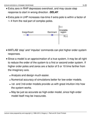
■ Extra zero in LHP will increase overshoot if the zero is within a factor
of ≈ 4 from the real part of complex poles.
Lecture notes prepared by and copyright c⃝ 1998–2013, Gregory L. Plett and M. Scott Trimboli](https://image.slidesharecdn.com/ece4510-notes03-170714151943/85/Ece4510-notes03-24-320.jpg)
![ECE4510/ECE5510, DYNAMIC RESPONSE 3–26
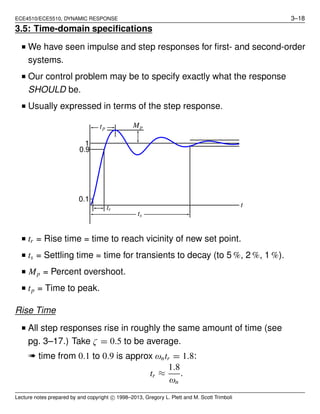
3.7: Changing dynamic response
■ Topic of the rest of the course.
■ Important tool: block diagram manipulation.
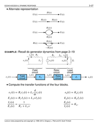
Block-diagram manipulation
■ We have already seen block diagrams (see pg. 1–4).
■ Shows information/energy flow in a system, and when used with
Laplace transforms, can simplify complex system dynamics.
■ Four BASIC configurations:
H(s) Y(s)U(s) Y(s) = H(s)U(s)
H1(s) H2(s) Y(s)U(s) Y(s) = [H2(s)H1(s)]U(s)
H1(s)
H2(s)
Y(s)U(s) Y(s) = [H1(s) + H2(s)]U(s)
H1(s)
H2(s)
Y(s)R(s)
U1(s)
Y2(s) U2(s)
U1(s) = R(s) − Y2(s)
Y2(s) = H2(s)H1(s)U1(s)
so, U1(s) = R(s) − H2(s)H1(s)U1(s)
=
R(s)
1 + H2(s)H1(s)
Y(s) = H1(s)U1(s)
=
H1(s)
1 + H2(s)H1(s)
R(s)
Lecture notes prepared by and copyright c⃝ 1998–2013, Gregory L. Plett and M. Scott Trimboli](https://image.slidesharecdn.com/ece4510-notes03-170714151943/85/Ece4510-notes03-26-320.jpg)


![CHAPTER LAPLACE TRANSFORM [Được lưu tự động].pptx](https://cdn.slidesharecdn.com/ss_thumbnails/chapterlaplacetransformclutng-230102000908-d6e0e181-thumbnail.jpg?width=640&height=640&fit=bounds)


