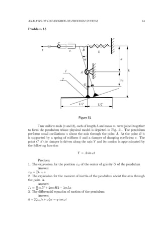
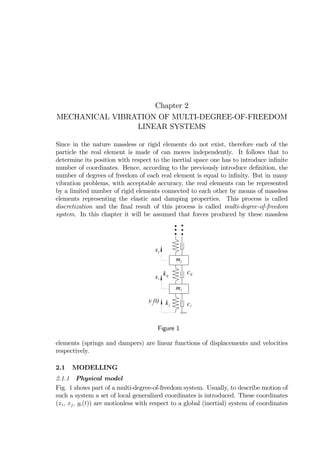
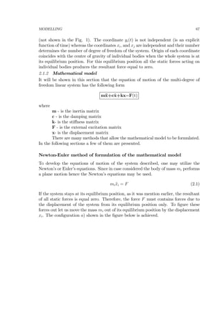
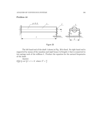
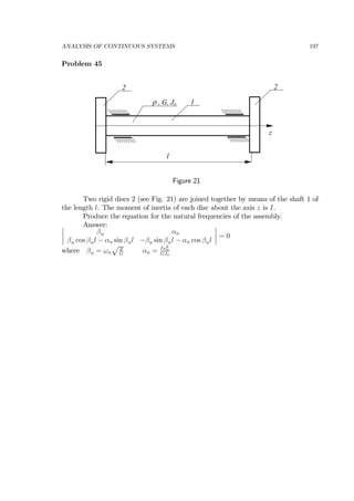
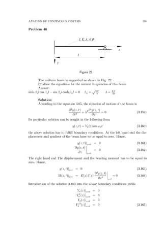
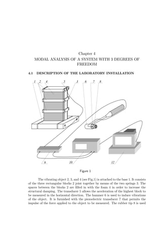
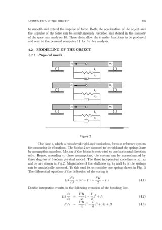
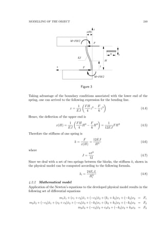
This document describes a textbook on mechanical vibration of linear systems. It covers modeling and analysis of one-degree-of-freedom and multi-degree-of-freedom linear systems, as well as continuous systems like strings, rods, shafts and beams. The textbook is divided into two parts, with part one covering modeling and analysis using mathematical techniques like Newton's laws, Lagrange's equations and influence coefficients. Part two describes laboratory experiments on modal analysis of multi-degree-of-freedom systems and vibration control techniques.


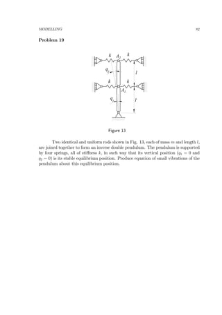
![ANALYSIS OF ONE-DEGREE-OF-FREEDOM SYSTEM 29
into the equation 1.34 results in two algebraic equation that are linear with respect
to the unknown constants Cs and Cc.
Cc = x0
Csωn = v0 (1.35)
According to 1.34, the particular solution that represents the free vibration of the
system is
x =
v0
ωn
sin ωnt + x0 cos ωnt =
= C sin(ωnt + α) (1.36)
where
C =
s
(x0)2 +
µ
v0
ωn
¶2
; α = arctan
Ã
x0
v0
ωn
!
(1.37)
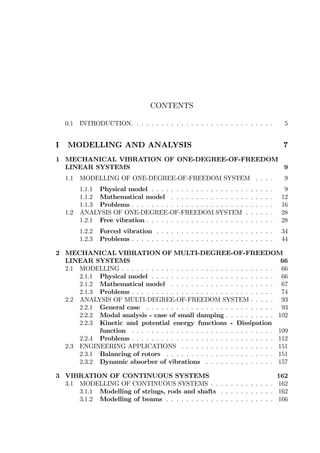
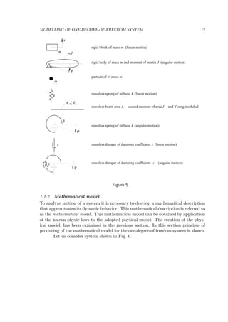
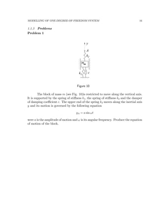
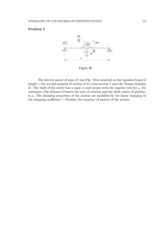
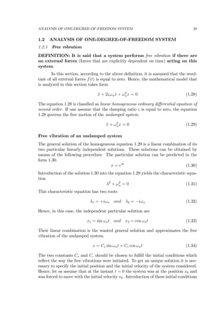
For ωn = 1[1/s], x0 = 1[m] v0 = 1[m/s] and ς = 0 the free motion is shown in Fig.
22 The free motion, in the case considered is periodic.
40
-1.5
-1
-0.5
0
0.5
1
10 20 30 50
x[m]
t[s]
C
Tn
α
xo
vo
Figure 22
DEFINITION: The shortest time after which parameters of motion repeat
themselves is called period and the motion is called periodic motion.
According to this definition, since the sine function has a period equal to 2π,
we have
sin(ωn(t + Tn) + α) = sin(ωnt + α + 2π) (1.38)](https://image.slidesharecdn.com/mechanicalvibrationbyjanuszkrodkiewski-130817083717-phpapp01/85/Mechanical-vibration-by-janusz-krodkiewski-29-320.jpg)
![ANALYSIS OF ONE-DEGREE-OF-FREEDOM SYSTEM 31
Introduction of the expressions 1.48 into 1.46 produces the free motion in the following
form
x = e−ςωnt
(Cs sin ωdt + Cc cos ωdt) = Ce−ςωnt
sin(ωdt + α) (1.49)
where
C =
sµ
v0 + ςωnx0
ωd
¶2
+ (x0)2
; α = arctan
x0ωd
v0 + ςωnx0
; ωd = ωn
p
1 − ς2
(1.50)
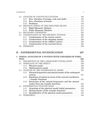
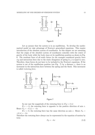
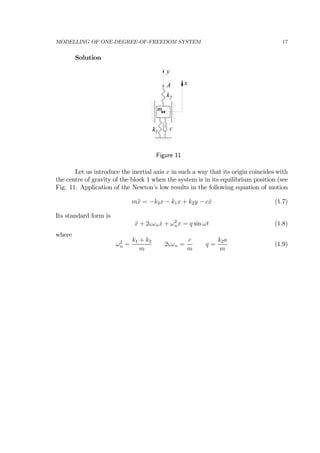
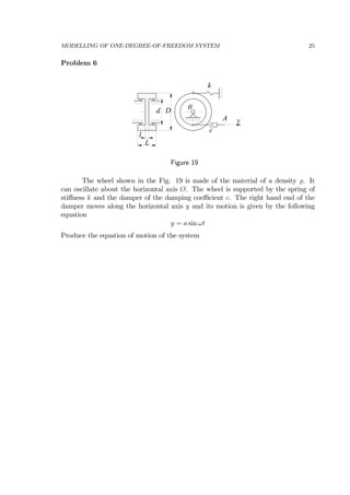
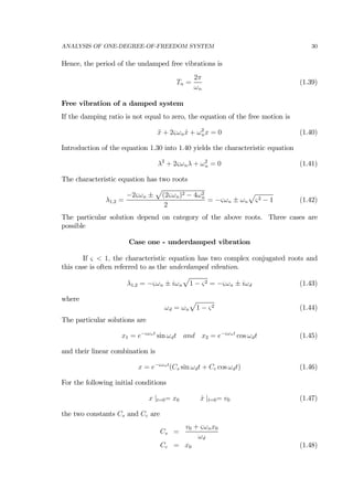
For ωn = 1[1/s], x0 = 1[m] v0 = 1[m/s] and ς = .1 the free motion is shown in Fig.
23In this case the motion is not periodic but the time Td (see Fig. 23) between every
-1.5
-1
-0.5
0
0.5
1
10 20 30 40 50
x[m]
t[s]
Td
Td
x(t)x(t+ Td
t
xo
vo
)
Figure 23
second zero-point is constant and it is called period of the dumped vibration. It is easy
to see from the expression 1.49 that
Td =
2π
ωd
(1.51)
DEFINITION: Natural logarithm of ratio of two displacements x(t) and
x(t + Td) that are one period apart is called logarithmic decrement of damping
and will be denoted by δ.](https://image.slidesharecdn.com/mechanicalvibrationbyjanuszkrodkiewski-130817083717-phpapp01/85/Mechanical-vibration-by-janusz-krodkiewski-31-320.jpg)
![ANALYSIS OF ONE-DEGREE-OF-FREEDOM SYSTEM 32
It will be shown that the logaritmic decrement is constant. Indeed
δ = ln
x (t)
x (t + Td)
= ln
Ce−ςωnt
sin(ωdt + α)
Ce−ςωn(t+Td) sin(ωd(t + Td) + α)
=
= ln
Ce−ςωnt
sin(ωdt + α)
Ce−ςωnte−ςωnTd sin(ωdt + 2π + α)
= ςωnTd =
2πςωn
ωd
=
2πςωn
ωn
√
1 − ς2
=
=
2πς
√
1 − ς2
(1.52)
This formula is frequently used for the experimental determination of the damping
ratio ς.
ς =
δ
p
4π2 + δ2
(1.53)
The other parameter ωn that exists in the mathematical model 1.40 can be easily
identified by measuring the period of the free motion Td. According to the formula
1.44 and 1.51
ωn =
ωd
√
1 − ς2
=
2π
Td
√
1 − ς2
(1.54)
Case two - critically damped vibration
If ς = 1, the characteristic equation has two real and equal one to each other
roots and this case is often referred to as the critically damped vibration
λ1,2 = −ςωn (1.55)
The particular solutions are
x1 = e−ςωnt
and x2 = te−ςωnt
(1.56)
and their linear combination is
x = Cse−ςωnt
+ Ccte−ςωnt
(1.57)
For the following initial conditions
x |t=0= x0 ˙x |t=0= v0 (1.58)
the two constants Cs and Cc are as follow
Cs = x0
Cc = v0 + x0ωn (1.59)
Introduction of the expressions 1.59 into 1.57 produces expression for the free motion
in the following form
x = e−ςωnt
(x0 + t(v0 + x0ωn)) (1.60)
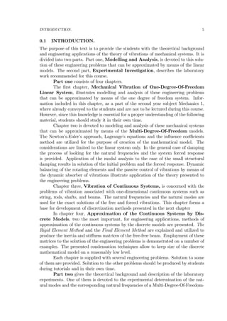
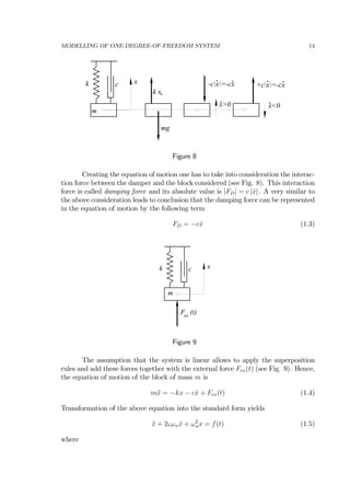
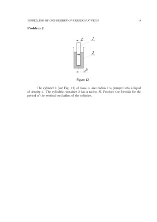
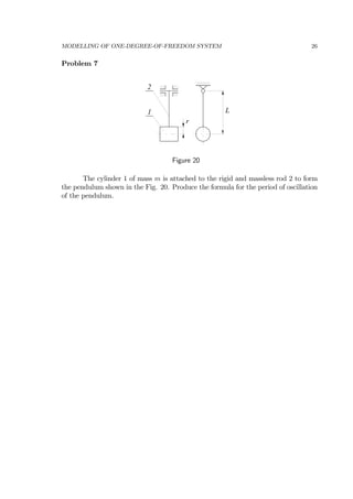
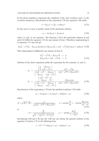
For ωn = 1[1/s], x0 = 1[m] v0 = 1[m/s] and ς = 1. the free motion is shown in
Fig. 24. The critical damping offers for the system the possibly faster return to its
equilibrium position.](https://image.slidesharecdn.com/mechanicalvibrationbyjanuszkrodkiewski-130817083717-phpapp01/85/Mechanical-vibration-by-janusz-krodkiewski-32-320.jpg)
![ANALYSIS OF ONE-DEGREE-OF-FREEDOM SYSTEM 33
-1.5
-1
-0.5
0
0.5
1
10 20 30 40 50
x[m]
t[s]
vo
xo
Figure 24
Case three - overdamped vibration
If ς > 1, the characteristic equation has two real roots and this case is often
referred to as the overdamped vibration.
λ1,2 = −ςωn ± ωn
p
ς2 − 1 = ωn(−ς ±
p
ς2 − 1) (1.61)
The particular solutions are
x1 = e−ωn(ς+
√
ς2−1)t
and x2 = e−ωn(ς−
√
ς2−1)t
(1.62)
and their linear combination is
x = e−ωnt
³
Cseωn
√
ς2−1)t
+ Cce−ωn
√
ς2−1)t
´
(1.63)
For the following initial conditions
x |t=0= x0 ˙x |t=0= v0 (1.64)
the two constants Cs and Cc are as follow
Cs =
+ v0
ωn
+ x0(+ς +
√
ς2 − 1)
2
√
ς2 − 1
Cc =
− v0
ωn
+ x0(−ς +
√
ς2 − 1)
2
√
ς2 − 1
(1.65)
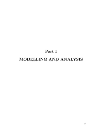
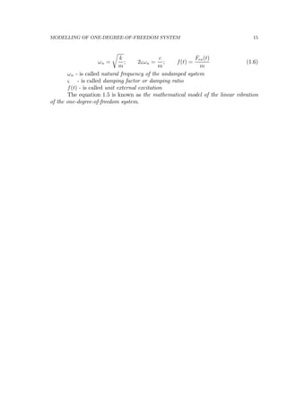
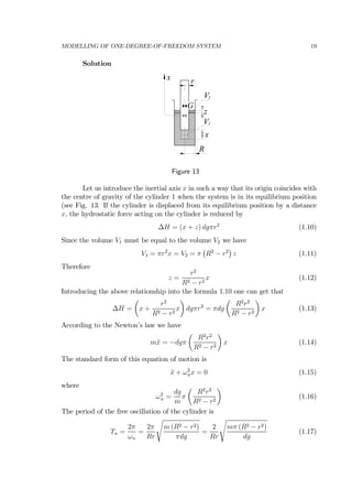
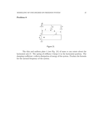
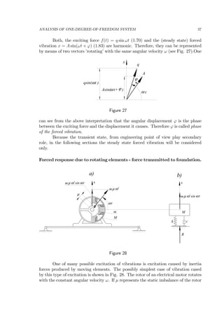
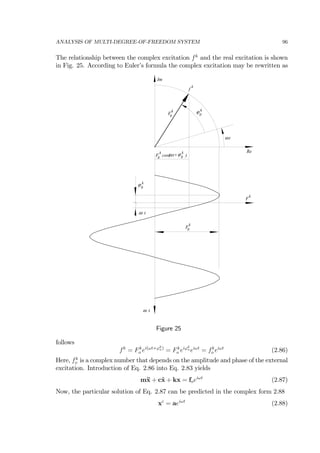
For ωn = 1[1/s], x0 = 1[m] v0 = 1[m/s] and ς = 5. the free motion is shown in Fig.
25](https://image.slidesharecdn.com/mechanicalvibrationbyjanuszkrodkiewski-130817083717-phpapp01/85/Mechanical-vibration-by-janusz-krodkiewski-33-320.jpg)
![ANALYSIS OF ONE-DEGREE-OF-FREEDOM SYSTEM 34
-1.5
-1
-0.5
0
0.5
1
10 20 30 40 50
x[m]
t[s]
vo
xo
Figure 25
1.2.2 Forced vibration
In a general case motion of a vibrating system is due to both, the initial conditions and
the exciting force. The mathematical model, according to the previous consideration,
is the linear non-homogeneous differential equation of second order.
¨x + 2ςωn ˙x + ω2
nx = f(t) (1.66)
where
ωn =
r
k
m
; 2ςωn =
c
m
; f(t) =
Fex(t)
m
(1.67)
The general solution of this mathematical model is a superposition of the general
solution of the homogeneous equation xg and the particular solution of the non-
homogeneous equation xp.
x = xg + xp (1.68)
The general solution of the homogeneous equation has been produced in the previous
section and for the underdamped vibration it is
xg = e−ςωnt
(Cs sin ωdt + Cc cos ωdt) = Ce−ςωnt
sin(ωdt + α) (1.69)
To produce the particular solution of the non-homogeneous equation, let as assume
that the excitation can be approximated by a harmonic function. Such a case is
referred to as the harmonic excitation.
f(t) = q sin ωt (1.70)](https://image.slidesharecdn.com/mechanicalvibrationbyjanuszkrodkiewski-130817083717-phpapp01/85/Mechanical-vibration-by-janusz-krodkiewski-34-320.jpg)
![ANALYSIS OF ONE-DEGREE-OF-FREEDOM SYSTEM 36
The constants C and α should be chosen to fullfil the required initial conditions.
For the following initial conditions
x |t=0= x0 ˙x |t=0= v0 (1.80)
one can get the following set of the algebraic equations for determination of the
parameters C and α
x0 = Co sin αo + A sin ϕ
v0 = −Coςωn sin αo + Coωd cos αo + Aω cos ϕ (1.81)
Introduction of the solution of the equations 1.81 (Co,αo) to the general solution,
yields particular solution of the non-homogeneous equation that represents the forced
vibration of the system considered.
x = Coe−ςωnt
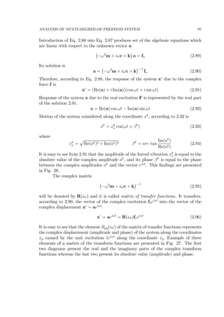
sin(ωdt + αo) + A sin(ωt + ϕ) (1.82)
This solution, for the following numerical data ς = 0.1, ωn = 1[1/s], ω = 2[1/s],
Co = 1[m], αo = 1[rd], A = 0.165205[m], ϕ = 0.126835[rd] is shown in Fig. 26
(curve c).The solution 1.82 is assembled out of two terms. First term represents an
-0.6
-0.4
-0.2
0
0.2
0.4
0.6
0.8
1
20 40 60
x[m]
t[s]
transient state of the forced vibration steady state of the forced vibration
abc
A
Figure 26
oscillations with frequency equal to the natural frequency of the damped system ωd.
Motion represented by this term, due to the existing damping, decays to zero (curve
a in Fig. 1.82) and determines time of the transient state of the forced vibrations.
Hence, after an usually short time, the transient state changes into the steady state
represented by the second term in equation 1.82 (curve b in Fig. 1.82)
x = A sin(ωt + ϕ) (1.83)
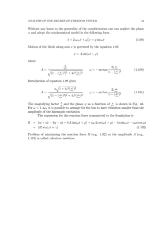
This harmonic term has amplitude A determined by the formula 1.77. It does not
depend on the initial conditions and is called amplitude of the forced vibration. Mo-
tion approximated by the equation 1.83 is usually referred to as the system forced
vibration.](https://image.slidesharecdn.com/mechanicalvibrationbyjanuszkrodkiewski-130817083717-phpapp01/85/Mechanical-vibration-by-janusz-krodkiewski-36-320.jpg)
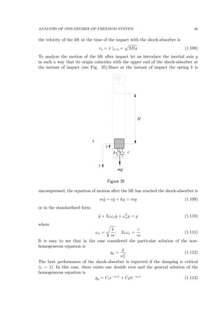
![ANALYSIS OF ONE-DEGREE-OF-FREEDOM SYSTEM 49
displacement
time [s]
y [m]
0
0.5
1
1.5
2
2.5
0 0.25 0.5 0.75 1
v [m/s]
velocity
time [s]
-5
0
5
10
15
20
25
0.25 0.5 0.75 1
acceleration
time [s]
-200
-150
-100
-50
0
50
0.25 0.5 0.75 1
a [m/s ]2
Figure 36](https://image.slidesharecdn.com/mechanicalvibrationbyjanuszkrodkiewski-130817083717-phpapp01/85/Mechanical-vibration-by-janusz-krodkiewski-49-320.jpg)
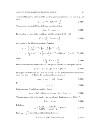
![ANALYSIS OF ONE-DEGREE-OF-FREEDOM SYSTEM 51
431 2
time [s]
-0.003
-0.002
-0.001
0
0.001
0.002
0.003
x[m]
Figure 39
Answer
m = 7000kg; k = 3000000Nm−1
; c = 15000Nsm−1](https://image.slidesharecdn.com/mechanicalvibrationbyjanuszkrodkiewski-130817083717-phpapp01/85/Mechanical-vibration-by-janusz-krodkiewski-51-320.jpg)
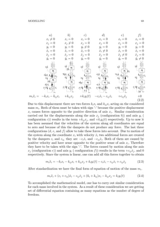

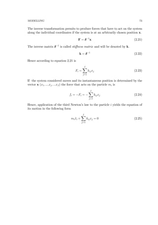
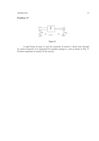
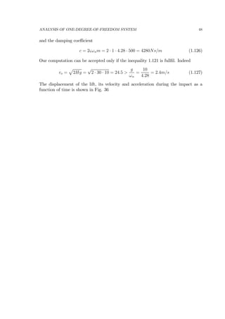
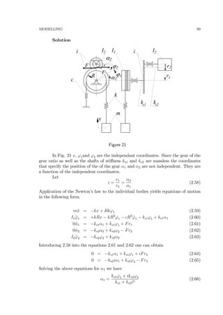
![MODELLING 78
Solution.
k
G
y
1
l1 l2
k2
y
ϕ
y =y+ϕ l22ϕ l11
O
F
M
y =y-
Figure 10
The system has two degree of freedom. Let us then introduce the two coordi-
nates y and ϕ as shown in Fig. 10.
The force F and the moment M that act on the beam due to its motion along
coordinates y and ϕ are
F = −y1k1 − y2k2 = −(y − ϕl1)k1 − (y + ϕl2)k2
= −[(k1 + k2)y + (k2l2 − k1l1)ϕ]
M = +y1k1l1 − y2k2l2 = +(y − ϕl1)k1l1 − (y + ϕl2)k2l2
= −[(k2l2 − k1l1)y + (k1l2
1 + yk2l2
2)ϕ (2.37)
Hence, the generalized Newton’s equations yield
m¨y = F = −[(k11 + k2)y + (k2l2 − k1l1)ϕ]
I ¨ϕ = M = −[(k2l2 − k1l1)y + (k1l2
1 + yk2l2
2)ϕ (2.38)
The matrix form of the system equations of motion is
m¨x + kx = 0 (2.39)
where
m =
∙
m 0
0 I
¸
; k =
∙
k1 + k2 k2l2 − k1l1
k2l2 − k1l1 k1l2
1 + k2l2
2
¸
; x =
∙
y
ϕ
¸
(2.40)](https://image.slidesharecdn.com/mechanicalvibrationbyjanuszkrodkiewski-130817083717-phpapp01/85/Mechanical-vibration-by-janusz-krodkiewski-78-320.jpg)
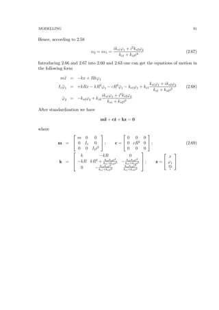
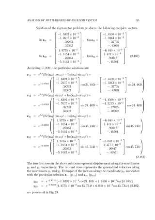
![ANALYSIS OF MULTI-DEGREE-OF-FREEDOM SYSTEM 94
corresponds to the case when the excitation F(t) is not present. Therefore, its gen-
eral solution represents the free (natural) vibrations of the system. The particular
solution of the non-homogeneous equation 2.70 represents the vibrations caused by
the excitation force F(t). It is often refered to as the forced vibrations.
Free vibrations - natural frequencies- stability of the equilibrium position
To analyze the free vibrations let us transfer the homogeneous equation 2.72 to so
called state-space coordinates. Let
y = ˙x (2.73)
be the vector of the generalized velocities. Introduction of Eq. 2.73 into Eq. 2.72
yields the following set of the differential equations of first order.
˙x = y
˙y = −m−1
kx − m−1
cy (2.74)
The above equations can be rewritten as follows
˙z = Az (2.75)
where
z =
∙
x
y
¸
, A =
∙
0 1
−m−1
k −m−1
c
¸
(2.76)
Solution of the above equation can be predicted in the form 2.77.
z = z0ert
(2.77)
Introduction of Eq. 2.77 into Eq. 2.75 results in a set of the homogeneous algebraic
equations which are linear with respect to the vector z0.
[A − 1r] z0 = 0 (2.78)
The equations 2.78 have non-zero solution if and only if the characteristic determinant
is equal to 0.
|[A − 1r]| = 0 (2.79)
The process of searching for a solution of the equation 2.79 is called eigenvalue problem
and the process of searching for the corresponding vector z0 is called eigenvector
problem. Both of them can be easily solved by means of the commercially available
computer programs.
The roots rn are usually complex and conjugated.
rn = hn ± iωn n = 1.....N (2.80)
Their number N is equal to the number of degree of freedom of the system considered.
The particular solutions corresponding to the complex roots 2.80 are
zn1 = ehnt
(Re(z0n) cos ωnt − Im(z0n) sin ωnt)
zn2 = ehnt
(Re(z0n) sin ωnt + Im(z0n) cos ωnt) n = 1.....N (2.81)](https://image.slidesharecdn.com/mechanicalvibrationbyjanuszkrodkiewski-130817083717-phpapp01/85/Mechanical-vibration-by-janusz-krodkiewski-94-320.jpg)
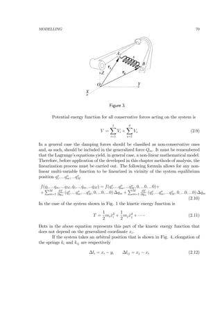
![ANALYSIS OF MULTI-DEGREE-OF-FREEDOM SYSTEM 95
In the above expressions Re(z0n ) and Im(z0n ) stand for the real and imaginary part
of the complex and conjugated eigenvector z0n associated with the nth
root of the
set 2.80 respectively. The particular solutions 2.81 allow to formulate the general
solution that approximates the system free vibrations..
z = [z11, z12,z21, z22,z31, z32,.....zn1, zn2,.........zN1, zN2] C (2.82)
As one can see from the formulae 2.81, the imaginary parts of roots rn represent
the natural frequencies of the system and their real parts represent rate of
decay of the free vibrations. The system with N degree of freedom possesses
N natural frequencies. The equation 2.82 indicates that the free motion of a multi-
degree-of-freedom system is a linear combination of the solutions 2.81.
A graphical interpretation of the solutions 2.81 is given in Fig. 24 for the
positive and negative magnitude of hn.The problem of searching for the vector of the
-20
-15
-10
-5
0
5
10
15
20
25
30
0.1 0.2 0.3 0.4 0.5 0.6 0.7 0.8 0.9 1 1.1 1.2 1.3 1.4 1.5 1.6 t
z
h>0
/π ω nnT = 2
-0.8
-0.6
-0.4
-0.2
0
0.2
0.4
0.6
0.8
1
0.1 0.2 0.3 0.4 0.5 0.6 0.7 0.8 0.9 1 1.1 1.2 1.3 1.4 1.5 1.6 t
z
/π ω nnT = 2
h<0
Figure 24
constant magnitudes C is called initial problem. In the general case, this problem is
difficult and goes beyond the scope of this lectures.
The roots 2.80 allow the stability of the system equilibrium position to be
determined.
If all roots rn of the equation 2.80 have negative real parts then the
equilibrium position of the system considered is stable.
If at least one root of the equation 2.80 has positive real part then
the equilibrium position of the system considered is unstable.
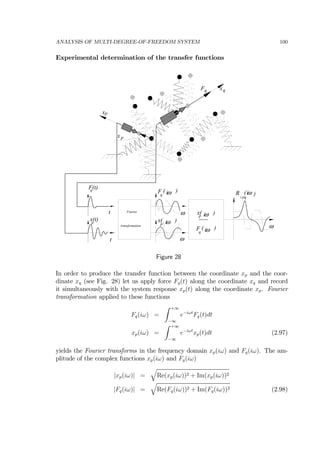
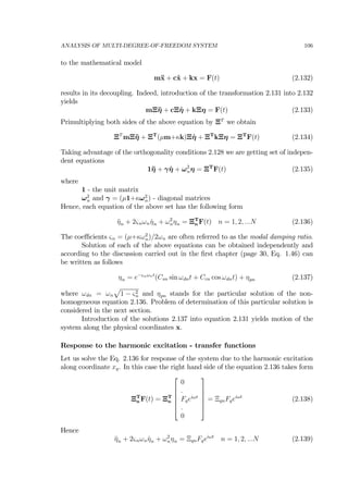
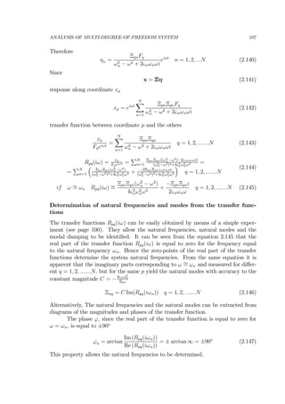
Forced vibrations - transfer functions
The response to the external excitation F(t) of a multi-degree-of-freedom system is
determined by the particular solution of the mathematical model 2.70.
m¨x + c˙x + kx = F(t) (2.83)
Let us assume that the excitation force F(t) is a sum of K addends. For the further
analysis let us assume that each of them has the following form
Fk
= Fk
o cos(ωt + ϕk
o) (2.84)
To facilitate the process of looking for the particular solution of equation 2.83, let us
introduce the complex excitation force by adding to the expression 2.84 the imaginary
part.
fk
= Fk
o cos(ωt + ϕk
o) + iFk
o sin(ωt + ϕk
o) (2.85)](https://image.slidesharecdn.com/mechanicalvibrationbyjanuszkrodkiewski-130817083717-phpapp01/85/Mechanical-vibration-by-janusz-krodkiewski-95-320.jpg)
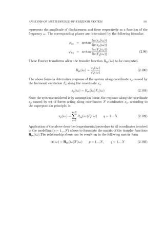
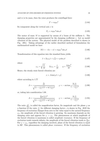
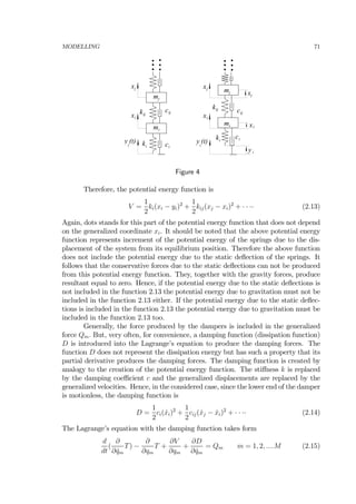
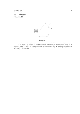
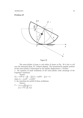
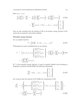
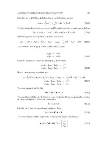
![ANALYSIS OF MULTI-DEGREE-OF-FREEDOM SYSTEM 103
frequency ωn. It determines the shape that the system must possess to oscillate
harmonically with the frequency ωn.
For example, if a beam with four concentrated masses is considered (see Fig.
29) the vector Xn contains four numbers
Xn = [X1n, X2n, X3n, X4n]T
(2.112)
If the system is deflected according to the this vector and allowed to move with the
Tn
X1n
X2n
X3n
X4n
x
3nx = X cos t3n ωn
t
Figure 29
initial velocity equal to zero, it will oscillate with the frequency ωn. There are four
such a natural modes and four corresponding natural frequencies for this system.
The problem of the determination of the natural frequencies is called eigen-
value problem and searching for the corresponding natural modes is called eigenvector
problem. Therefore the natural frequencies are very often referred to as eigenvalue
and the natural modes as eigenvectors.
Now, one can say that the process of determination of the particular solution
xn= Xn cos ωnt (2.113)
of the equation 2.105 has been accomplished. There are N such particular solutions.
In similar manner one can prove that
xn= Xn sin ωnt (2.114)
is a particular solution too. Since the solutions ?? and 2.114 are linearly independent,
their linear combination forms the general solution of the equation 2.105
xn =
NX
n=1
(SnXn sin ωnt + CnXn cos ωnt) (2.115)
The 2N constants Sn and Cn should be chosen to satisfy the 2N initial conditions.](https://image.slidesharecdn.com/mechanicalvibrationbyjanuszkrodkiewski-130817083717-phpapp01/85/Mechanical-vibration-by-janusz-krodkiewski-103-320.jpg)
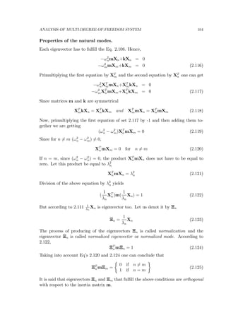
![ANALYSIS OF MULTI-DEGREE-OF-FREEDOM SYSTEM 105
Owning to the above orthogonality condition, the second of the equations
2.117 yields
ΞT
n kΞm =
½
0 if n 6= m
ω2
n if n = m
¾
(2.126)
It means that the normalized modes are orthogonal with respect to the matrix of
stiffness.
The modal modes Ξn can be arranged in a square matrix of order N known
as the modal matrix Ξ .
Ξ = [Ξ1, Ξ2, .....Ξn, ......ΞN ] where N is number of degrees of freedom (2.127)
It is easy to see that the developed orthogonality conditions yields
ΞT
mΞ = 1
ΞT
kΞ = ω2
(2.128)
where ω2
is a square diagonal matrix containing the squared natural frequencies ω2
n
ω2
=
⎡
⎢
⎢
⎢
⎢
⎢
⎢
⎣
ω2
1 0 . 0 . 0
0 ω2
2 . 0 . 0
. . . . . .
0 0 . ω2
n . 0
. . . . . .
0 0 . 0 . ω2
N
⎤
⎥
⎥
⎥
⎥
⎥
⎥
⎦
(2.129)
Normal coordinates - modal damping
Motion of any real system is always associated with a dissipation of energy. Vibrations
of any mechanical structures are coupled with deflections of the elastic elements.
These deflections, in turn, cause friction between the particles the elements are made
of. The damping caused by such an internal friction and damping due to friction of
these elements against the surrounding medium is usually referred to as the structural
damping. In many cases, particularly if the system considered is furnished with
special devices design for dissipation of energy called dampers, the structural damping
can be omitted. But in case of absence of such devices, the structural damping has
to be taken into account. The structural damping is extremely difficult or simply
impossible to be predicted by means of any analytical methods. In such cases the
matrix of damping c (see Eq. 2.104) is assumed as the following combination of the
matrix of inertia m and stiffness k with the unknown coefficients µ and κ.
c =µm+κk (2.130)
This coefficients are to be determined experimentally.
It will be shown that application of the following linear transformation
x = Ξη (2.131)](https://image.slidesharecdn.com/mechanicalvibrationbyjanuszkrodkiewski-130817083717-phpapp01/85/Mechanical-vibration-by-janusz-krodkiewski-105-320.jpg)

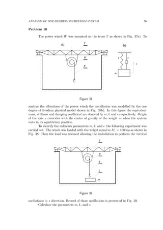
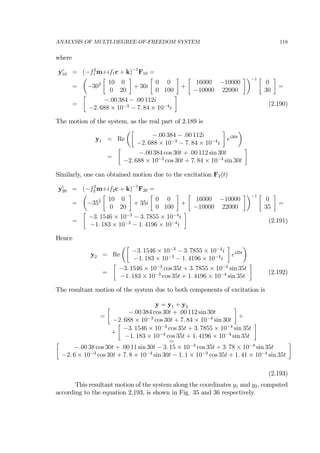
![ANALYSIS OF MULTI-DEGREE-OF-FREEDOM SYSTEM 116
t[s]43210
0.01
-0.01
-0.02
y111[m]
t[s]4320
0.01
-0.01
-0.02
y211[m]
1
Figure 33](https://image.slidesharecdn.com/mechanicalvibrationbyjanuszkrodkiewski-130817083717-phpapp01/85/Mechanical-vibration-by-janusz-krodkiewski-116-320.jpg)
![ANALYSIS OF MULTI-DEGREE-OF-FREEDOM SYSTEM 117
3. The steady state motion of the system due to the kinematic excitation
According to the given data, motion of the point A is
y = 0.01 · sin(30 · t) + 0.01 · sin(35 · t) (2.183)
t[s]1.510.5
y[m]
0.01
0
-0.01
-0.02
Figure 34
The time history diagram of this motion is given in Fig. 34
The particular solution y, which represents the forced vibration, according to
the superposition rule, is
y = y1 + y2 (2.184)
where y1 is the particular solution of the equation 2.185
m¨y + c˙y + ky = F1(t) (2.185)
and y2 is the particular solution of the equation 2.186
m¨y + c˙y + ky = F2(t) (2.186)
To produce the particular solution of the equation 2.185 let us introduce the complex
excitation
Fc
1(t) =
∙
0
a1 cos(f1t) + ia1 sin(f1t)
¸
=
∙
0
a1eif1t
¸
=
∙
0
a1
¸
eif1t
=
= F10eif1t
=
∙
0
30
¸
ei30t
(2.187)
Hence the equation of motion takes form
m¨y + c˙y + ky = F10eif1t
(2.188)
Its particular solution is
yc
1 = yc
10eif1t
(2.189)](https://image.slidesharecdn.com/mechanicalvibrationbyjanuszkrodkiewski-130817083717-phpapp01/85/Mechanical-vibration-by-janusz-krodkiewski-117-320.jpg)
![ANALYSIS OF MULTI-DEGREE-OF-FREEDOM SYSTEM 119
t[s]1.510.5
y1[m]
0.005
0
-0.005
-0.01
Figure 35
t[s]1.510.5
0.005
0
-0.005
-0.01
y2[m]
Figure 36](https://image.slidesharecdn.com/mechanicalvibrationbyjanuszkrodkiewski-130817083717-phpapp01/85/Mechanical-vibration-by-janusz-krodkiewski-119-320.jpg)
![ANALYSIS OF MULTI-DEGREE-OF-FREEDOM SYSTEM 120
4. The exciting force at the point A required to maintain the steady
state motion
m 2
A
c
y
y2
y2
y
.
.
Figure 37
To develop the expression for the force necessary to move the point A according
to the assumed motion 2.183, let us consider the damper c shown in Fig. 37. If the
point A moves with the velocity ˙y and in the same time the mass m2 moves with the
velocity ˙y2, the relative velocity of the point A with respect to the mass m2 is
v = ˙y − ˙y2 (2.194)
Therefore, to realize this motion, it is necessary to apply at the point A the following
force
FA = c ( ˙y − ˙y2) (2.195)
Hence, according to the equation 2.183 and 2.193 we have
FA = 100( d
dt
(0.01 · sin 30t + 0.01 · sin 35t) +
− d
dt
(−2. 6 · 10−3
cos 30t + 7. 8 · 10−4
sin 30t+
−1. 1 · 10−3
cos 35t + 1. 4 · 10−4
sin 35t)) =
= 27. 648 cos 30t + 34. 503 cos 35t − 8. 064 sin 30t − 4. 1405 sin 35t[N]
(2.196)
Diagram of this force is presented in Fig.38](https://image.slidesharecdn.com/mechanicalvibrationbyjanuszkrodkiewski-130817083717-phpapp01/85/Mechanical-vibration-by-janusz-krodkiewski-120-320.jpg)
![ANALYSIS OF MULTI-DEGREE-OF-FREEDOM SYSTEM 121
t[s]1.510.5
FA[N]
40
20
0
-20
-40
-60
Figure 38
5. The reaction force and the reaction moment at the point B.
RB
M B
P
J1l 1 E1
B
y1
Figure 39
According to Fig. 39
RB = P
MB = Pl1 (2.197)
where P is dependent on the instantaneous displacement y1. This relationship is
determined by the formula 2.173
P = k1y1 =
3E1J1
l3
1
y1 =
3 · 0.2 · 1012
· 1 · 10−8
13
= 6000y1 (2.198)
The motion along the coordinate y1 is determined by the function 2.193
y1 = −.00 38 cos 30t+.00 11 sin 30t−3. 15×10−3
cos 35t+3. 78×10−4
sin 35t (2.199)
Hence
RB=6000
¡
−.00 38 cos 30t+.00 11 sin 30t−3. 15×10−3
cos 35t + 3. 78×10−4
sin 35t
¢
MB=6000·1·
¡
−.00 38 cos 30t+.00 11 sin 30t−3. 15×10−3
cos 35t+3. 78×10−4
sin 35t
¢
(2.200)](https://image.slidesharecdn.com/mechanicalvibrationbyjanuszkrodkiewski-130817083717-phpapp01/85/Mechanical-vibration-by-janusz-krodkiewski-121-320.jpg)
![ANALYSIS OF MULTI-DEGREE-OF-FREEDOM SYSTEM 124
Solution
1. The natural frequencies and the natural modes
According to the given numerical data the moment of inertia of the ball, the
inertia matrix and the stuffiness matrix are
I =
2
5
· 1 · 0.052
= 0.001 kgm2
m =
∙
2 + 1 1 · 0.1
1 · 0.1 1 · 0.12
+ 0.001
¸
=
∙
3.0 . 1
. 1 .0 11
¸
(2.203)
k =
∙
1000 0
0 1 · 10 · 0.1
¸
=
∙
1000.0 0
0 1.0
¸
According to 2.108 (page 102) one can write the following set of equations
(−ω2
nm + k)X = 0 (2.204)
where ω stands for the natural frequency and X is the corresponding natural mode.
Hence for the given numerical data we are getting
∙
−3.0ω2
n + 1000.0 −. 1ω2
n
−. 1ω2
n −.0 11ω2
n + 1.0
¸ ∙
X
Φ
¸
=
∙
0
0
¸
(2.205)
This set of equations has non-zero solution if and only if its determinant is equal to
zero. Hence the equation for the natural frequencies is.
¯
¯
¯
¯
∙
−3.0ω2
n + 1000.0 −. 1ω2
n
−. 1ω2
n −.0 11ω2
n + 1.0
¸¯
¯
¯
¯ = .0 23ω4
n − 14.0ω2
n + 1000.0 = 0 (2.206)
Its roots: £
22. 936 −22. 936 9. 091 3 −9. 091 3
¤
yield the wanted natural frequencies
ω1 = 9. 0913 ω2 = 22. 936 [s−1
] (2.207)
For ωn = ω1 = 9. 0913 the equations 2.205 become linearly dependent. Therefore,
one of the unknown can be chosen arbitrarily (e.g. X1 = 1) and the other may be
produced from the first equation of the set 2.205.
X1 = 1
−3.0X1ω2
1 + 1000.0X1 − . 1ω2
1Φ1 = 0 (2.208)
Φ1 =
1
. 1 · 9.09132
− 3.0 · 9.092
+ 1000.0) = 90.99
These two numbers form the first mode of vibrations corresponding to the first
natural frequency ω1.Similar consideration, carried out for the natural frequency
ω2 = 22. 936,yields the second mode.
X2 = 1
Φ2 =
1
. 1 · 22.9362
¡
−3.0 · 22.9362
+ 1000.0
¢
= −10.991 (2.209)](https://image.slidesharecdn.com/mechanicalvibrationbyjanuszkrodkiewski-130817083717-phpapp01/85/Mechanical-vibration-by-janusz-krodkiewski-124-320.jpg)
![ANALYSIS OF MULTI-DEGREE-OF-FREEDOM SYSTEM 125
Now, one can create the modal matrix
X = [X1, X2] =
∙
1 1
90.99 −10.991
¸
(2.210)
In this case the modal matrix has two eigenvectors X1 and X2.
X1 =
∙
1
90.99
¸
; X2 =
∙
1
−10.991
¸
(2.211)
2. Normalization of the natural modes
According to 2.121 the normalization factor is
XT
n mXn = λ2
n (2.212)
Hence
λ2
1 =
£
1 90. 99
¤
∙
3.0 . 1
. 1 .0 11
¸ ∙
1
90.99
¸
= 112. 27
λ1 =
√
112. 27 = 10. 596 (2.213)
Division of the eigenvector X1 by the factor λ1 yields the normalized mode Ξ1.
Ξ1 =
1
10. 596
∙
1
90.99
¸
=
∙
9. 4375 × 10−2
8. 5872
¸
(2.214)
Similar procedure allows the second normalized mode to be obtained
λ2
2 =
£
1 −10.991
¤
∙
3.0 . 1
. 1 .0 11
¸ ∙
1
−10.991
¸
= 2. 1306
λ2 =
√
2. 1306 = 1. 4597
Ξ2 =
1
1. 4597
∙
1
−10.991
¸
=
∙
. 68507
−7. 5296
¸
(2.215)
These two vectors forms the normalized modal matrix Ξ.
Ξ =
∙
9. 4375 × 10−2
. 68507
8. 5872 −7. 5296
¸
(2.216)
The normalized eigenvectors must be orthogonal with respect to both the inertia
matrix and the stiffness matrix. Indeed.
ΞT
mΞ =
=
∙
9. 4375 × 10−2
8. 5872
. 68507 −7. 5296
¸ ∙
3.0 . 1
. 1 .0 11
¸ ∙
9. 4375 × 10−2
. 68507
8. 5872 −7. 5296
¸
=
∙
1 0
0 1
¸
(2.217)](https://image.slidesharecdn.com/mechanicalvibrationbyjanuszkrodkiewski-130817083717-phpapp01/85/Mechanical-vibration-by-janusz-krodkiewski-125-320.jpg)
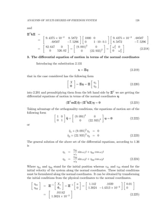
![ANALYSIS OF MULTI-DEGREE-OF-FREEDOM SYSTEM 127
∙
v01
v02
¸
=
∙
0
0
¸
(2.226)
Introduction of the above initial conditions into the equations 2.224 results in motion
of the system along the normal coordinates
η1 = η01 cos ω1t = .01142 cos 9.091t
η2 = η02 cos ω2t = 1.3024 × 10⁻²
cos 22.935t (2.227)
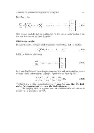
4. The equations of motion of the system along the coordinates x and ϕ
To produce equation of motion along the physical coordinates, one has to
transform the motion along the normal coordinates beck to the physical ones. Hence,
using the relationship 2.219, we are getting
∙
X
Φ
¸
= Ξη =
∙
9. 4375 × 10−2
. 68507
8. 5872 −7. 5296
¸ ∙
.01142 cos 9.091t
1.3024 × 10⁻²
cos 22.935t
¸
=
=
∙
1. 0778 × 10−3
cos 9. 091t + 8. 9224 × 10−3
cos 22. 935t
9. 8066 × 10−2
cos 9. 091t − 9. 8066 × 10−2
cos 22. 935t
¸
(2.228)
This motion is presented in Fig. 43 and 44
-0.01
-0.005
0
0.005
0.01
0.5 1 1.5 t[s]
X[m]
Figure 43
-0.15
-0.1
-0.05
0
0.05
0.1
0.15
0.2
0.5 1 1.5 t[s]
Φ [rad]
Figure 44](https://image.slidesharecdn.com/mechanicalvibrationbyjanuszkrodkiewski-130817083717-phpapp01/85/Mechanical-vibration-by-janusz-krodkiewski-127-320.jpg)
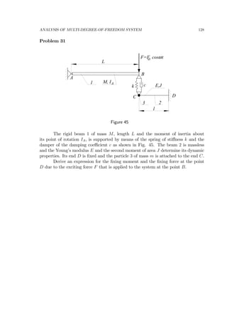

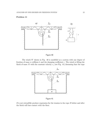
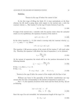
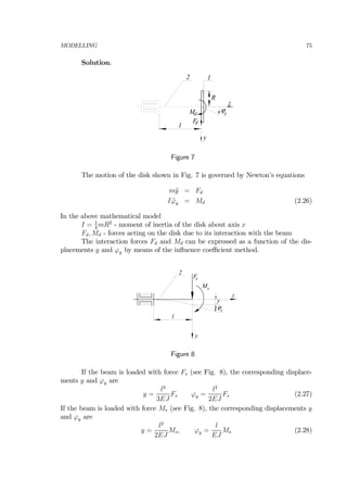
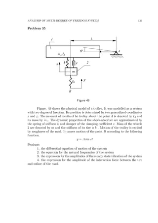
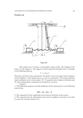
![ANALYSIS OF MULTI-DEGREE-OF-FREEDOM SYSTEM 132
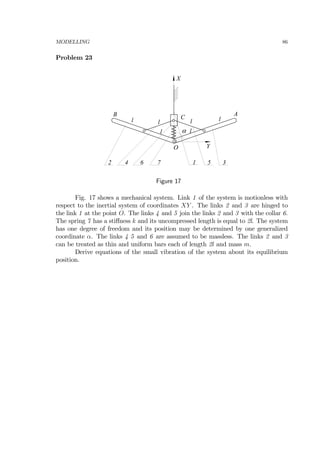
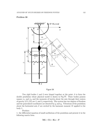
Problem 34
l l
C DA B
l
k
α
k
β
F
G
Figure 48
Three uniform platforms each of the length l, the mass m and the moment
of inertia about axis through its centre of gravity IG are hinged together to form a
bridge that is shown in Fig. 48. This bridge is supported by means of two springs
each of the stiffness k. This system has two degree of freedom and the two generalized
coordinates are denoted by α and β. There is an excitation force F applied at the
hinge C. This force can be adopted in the following form
F = Fo cos ωt
Produce:
1. the differential equations of motion of the system and present them in the standard
form
Answer:
M¨x + Kx = F
M =
∙ 2
3
−1
6
−1
6
2
3
¸
ml2
; K =
∙
1 0
0 1
¸
kl2
; x =
∙
α
β
¸
; F =
∙
0
Fol
¸
cos ωt
2. the equation for the natural frequencies of the system
Answer:
|K − 1ωn| = 0
3. the expression for the amplitude of the forced vibrations of the system
Answer:
X = [−ω2
M + K]
−1
∙
0
Fol
¸
cos ωt =
∙
A
B
¸
4. the expression for the interaction force between the spring attached to the hinge
B and the ground
Answer:
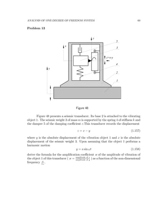
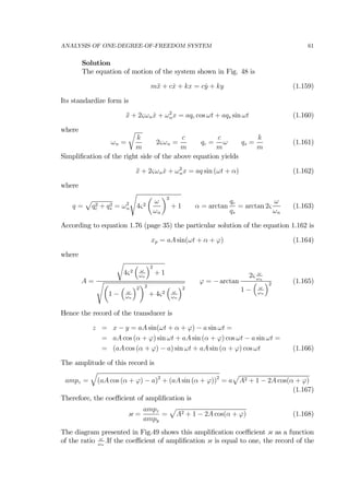
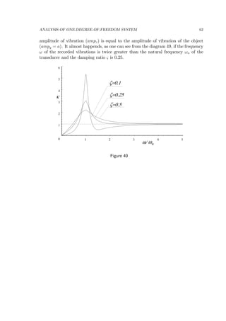
R = Akl cos ωt](https://image.slidesharecdn.com/mechanicalvibrationbyjanuszkrodkiewski-130817083717-phpapp01/85/Mechanical-vibration-by-janusz-krodkiewski-132-320.jpg)

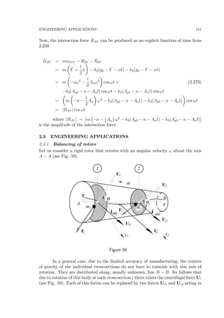
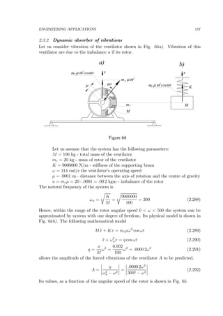
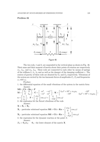
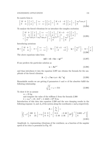
![ENGINEERING APPLICATIONS 158
0
0.0001
100 200 300 400
A1[m]
ω[ 1/s]
Figure 65
As it can be seen from this diagram, the ventilator develops large vibration in
vicinity of its working speed ω = 314 rad/s and has to pass the critical speed during
the run up. Such a solution is not acceptable. One of a possible way of reducing
these vibration is to furnish the ventilator with the absorber of vibration shown in
fig 66
x
µ ω t
m µ ω2
cosω t x
M
m
m µ ω 2
cosω t
M
K
m µ ω2
a) b)
ck
r
r
m
r
y
y
c
m
k
r
Figure 66
It comprises block of mass m, elastic element of stiffness k and damper of the
damping coefficient c. Application of the Newton’s - Euler’s method, results in the
following mathematical model.
M ¨x + (K + k)x − ky + c ˙x − c ˙y = uω2
cosωt
m¨y − kx + ky − c ˙x + c ˙y = 0 (2.293)](https://image.slidesharecdn.com/mechanicalvibrationbyjanuszkrodkiewski-130817083717-phpapp01/85/Mechanical-vibration-by-janusz-krodkiewski-158-320.jpg)
![ENGINEERING APPLICATIONS 160
0
0.0001
100 200 300 400
A1[m]
ω[1/s]
Figure 67
One can notice that the amplitude of vibration for the working speed ω = 314
rad/s is equal to zero. But the ventilator still has to pass resonance in vicinity of
ω = 240 rad/s. To improve the dynamic response, let us analyze the influence of the
damping coefficient c.
∙
A1
A2
¸
=
=
µ
−ω2
∙
100 0
0 25
¸
+ iω
∙
c c
c c
¸
103
+
∙
11.5 −2. 46
−2. 46 2. 46
¸
106
¶−1 ∙
0.002 · ω2
0
¸
(2.302)
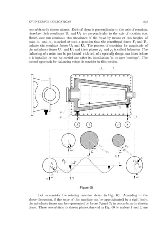
The amplitudes of the forced vibration of the ventilator for different values of the
damping coefficient c, computed according to the formula 2.302 are collected in the
Table 1. It can be noticed, that by increasing the damping coefficient c one can lower
amplitude of vibrations in all region of frequency. The best results of attenuation of
vibrations can be achieved if the two local maxima are equal to each other. This case
is shown in the last raw of the table 1. Application of the absorber of vibrations offers
a safe operation in region of the angular speed 0 < ω < 500 rad/s. The amplitude is
less than 0.00004 m. Damping coefficient lager then 5000 results in increment of the
amplitude of the ventilator’s forced vibrations. If the damping tends to infinity, The
relative motion is ceased and the system behaves like the undamped system with one
degree of freedom.](https://image.slidesharecdn.com/mechanicalvibrationbyjanuszkrodkiewski-130817083717-phpapp01/85/Mechanical-vibration-by-janusz-krodkiewski-160-320.jpg)
![ENGINEERING APPLICATIONS 161
.
Table 1
m = 25
k = 2. 46 × 106
c = 0
0
0.0001
100 200 300 400 ω[1/s]
A1[m]
m = 25
k = 2. 46 × 106
c = 1000
4003002001000
0.0001
0
A1[m]
ω[1/s]
m = 25
k = 2. 46 × 106
c = 2500
4003002001000
0.0001
0
A1[m]
ω[1/s]
m = 25
k = 2. 46 × 106
c = 5000
0
0.0001
100 200 300 400
0
A1[m]
ω[1/s
]
m = 25
k = 1.75 × 10⁶
c = 5000
0
0.0001
100 200 300 400
0
A1[m]
ω[1/s]](https://image.slidesharecdn.com/mechanicalvibrationbyjanuszkrodkiewski-130817083717-phpapp01/85/Mechanical-vibration-by-janusz-krodkiewski-161-320.jpg)
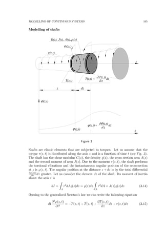
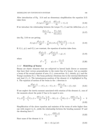
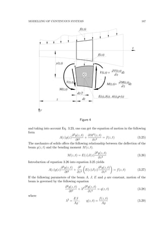
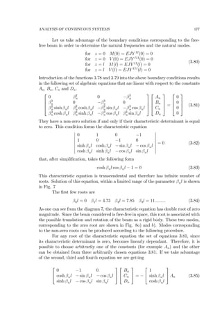
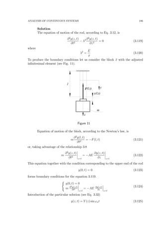
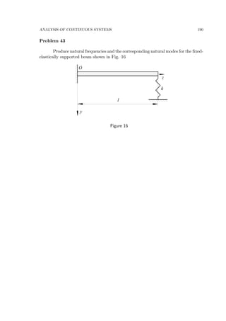
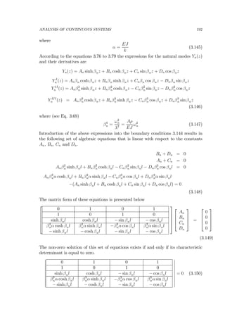
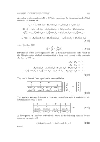
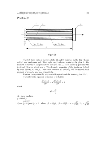
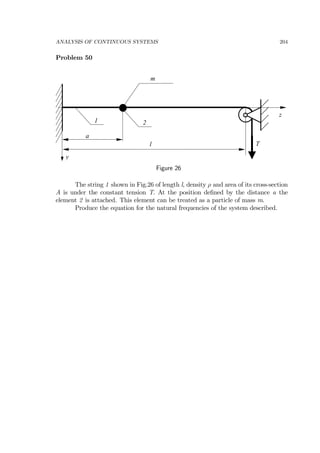
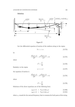
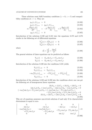
![ANALYSIS OF CONTINUOUS SYSTEMS 184
displacement and continuity of the torque. The last condition says that the torque
at the free end is zero. Since the general solution of equation 3.110 and 3.111are
Φ1(z) = Sn1 sin
ωn
λ1
z + Cn1 cos
ωn
λ1
z (3.114)
Φ2(z) = Sn2 sin
ωn
λ2
z + Cn2 cos
ωn
λ2
z (3.115)
the formulated boundary conditions results in the following set of equations
Cn1 = 0
Sn1 sin ωn
λ1
l1 + Cn1 cos ωn
λ1
l1 − Sn2 sin ωn
λ2
l2 − Cn2 cos ωn
λ2
l2 = 0
Sn1G1J1
ωn
λ1
cos ωn
λ1
l1 − Cn1G1J1
ωn
λ1
sin ωn
λ1
l1+
−Sn2G2J2
ωn
λ2
cos ωn
λ2
l1 + Cn2G2J2
ωn
λ2
sin ωn
λ2
l1 = 0
+Sn2
ωn
λ2
cos ωn
λ2
(l1 + l2) − Cn2
ωn
λ2
sin ωn
λ2
(l1 + l2) = 0
(3.116)
Its matrix for is
[A]
⎡
⎢
⎢
⎣
Sn1
Cn1
Sn2
Cn2
⎤
⎥
⎥
⎦ = 0 (3.117)
where
[A] =
⎡
⎢
⎢
⎣
0 1 0 0
sin ωn
λ1
l1 cos ωn
λ1
l1 − sin ωn
λ2
l2 − cos ωn
λ2
l2
G1J1
ωn
λ1
cos ωn
λ1
l1 −G1J1
ωn
λ1
sin ωn
λ1
l1 −G2J2
ωn
λ2
cos ωn
λ2
l1 G2J2
ωn
λ2
sin ωn
λ2
l1
0 0 ωn
λ2
cos ωn
λ2
(l1+l2) −ωn
λ2
sin ωn
λ2
(l1+l2)
⎤
⎥
⎥
⎦
This homogeneous set of equations has the non-zero solutions if and only if its char-
acteristic determinant is equal to zero.
¯
¯
¯
¯
¯
¯
¯
¯
0 1 0 0
sin ωn
λ1
l1 cos ωn
λ1
l1 − sin ωn
λ2
l2 − cos ωn
λ2
l2
G1J1
ωn
λ1
cos ωn
λ1
l1 −G1J1
ωn
λ1
sin ωn
λ1
l1 −G2J2
ωn
λ2
cos ωn
λ2
l1 G2J2
ωn
λ2
sin ωn
λ2
l1
0 0 ωn
λ2
cos ωn
λ2
(l1+l2) −ωn
λ2
sin ωn
λ2
(l1+l2)
¯
¯
¯
¯
¯
¯
¯
¯
= 0
(3.118)
Solution of this equation for the roots ωn yields the wanted natural frequencies of the
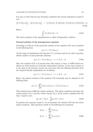
shaft.](https://image.slidesharecdn.com/mechanicalvibrationbyjanuszkrodkiewski-130817083717-phpapp01/85/Mechanical-vibration-by-janusz-krodkiewski-184-320.jpg)

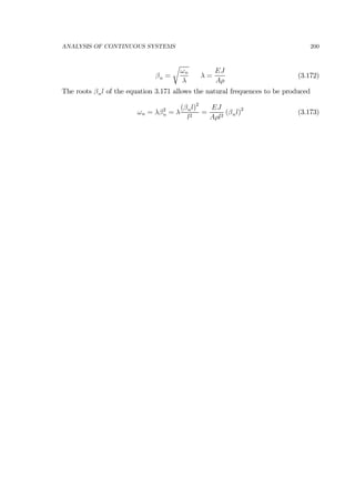

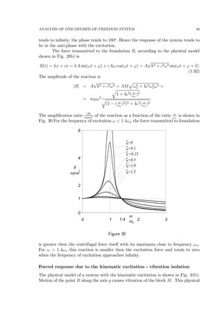
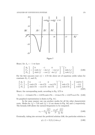
![ANALYSIS OF CONTINUOUS SYSTEMS 211
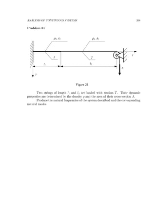
l1 = .5m, l2 = 1.m, 1 = 2 = 7800kg/m3
, A1 = 2 · 10−6
m2
, A2 = 1 · 10−6
m2
,
T = 500N.
λ1 =
q
T
A1ρ1
q
500
2·10−67800
= 179.03m/s, λ2 =
q
T
A2ρ2
=
q
500
1·10−67800
= 253.18m/s
¯
¯
¯
¯
¯
¯
¯
¯
0 1 0 0
sin
¡ .5
179
ωn
¢
cos
¡ .5
179
ωn
¢
− sin
¡ .5
253
ωn
¢
− cos
¡ .5
253
ωn
¢
1
179
cos
¡ .5
179
ωn
¢
− 1
179
sin
¡ .5
179
ωn
¢
− 1
253
cos
¡ .5
253
ωn
¢
+ 1
253
sin
¡ .5
253
ωn
¢
0 0 sin
¡ 1
253.
(.5 + 1.)ωn
¢
cos
¡ 1
253
(.5 + 1.)ωn
¢
¯
¯
¯
¯
¯
¯
¯
¯
= 0
(3.215)
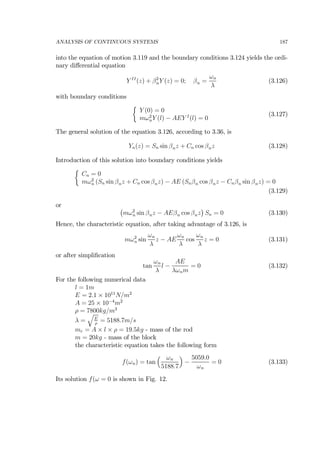
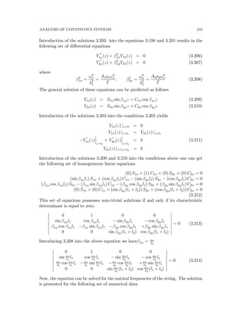
The magnitude of the determinant as a function of the frequency ωn is presented in
Fig. 29
25002000150010005000
10
5
0
-5
-10
frequency [rad/s]frequency [rad/s]
Figure 29
It allows the natural frequencies to be determined. They are
ω1 = 483; ω2 = 920; ω3 = 1437; ω4 = 1861; ω5 = 2344[rad/s] (3.216)
The so far unknown constants S1n, C1n, S2n, C2n can be computed from the homo-
geneous set of linear equations 3.212. From the first equation one can see that the
constant C1n must be equal to zero
C1n = 0
(sin β1nl1) S1n − (sin β2nl1) S2n − (cos β2nl1) C2n = 0
(β1n cos β1nl1) S1n − (β2n cos β2nl1) S2n + (β2n sin β2nl1) C2n = 0
(0) S1n + (sin β2n(l1 + l2)) S2n + (cos β2n(l1 + l2)) C2n = 0
(3.217)](https://image.slidesharecdn.com/mechanicalvibrationbyjanuszkrodkiewski-130817083717-phpapp01/85/Mechanical-vibration-by-janusz-krodkiewski-211-320.jpg)
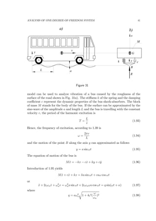
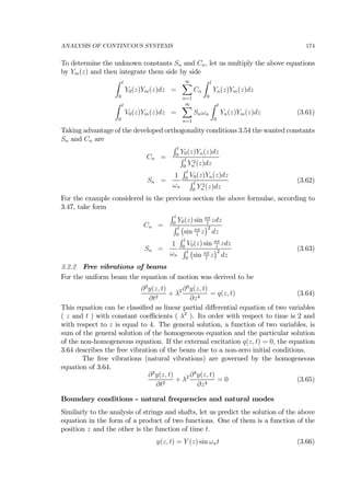
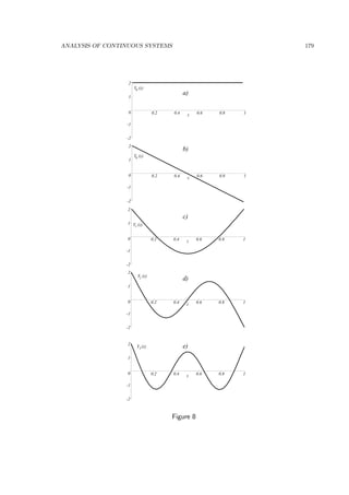
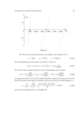
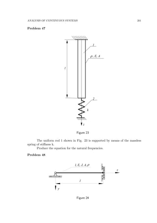
![ANALYSIS OF CONTINUOUS SYSTEMS 213
natural m odes
-2
-1
0
1
2
3
4
0 0.5 1 1.5
z [m ]
Figure 30](https://image.slidesharecdn.com/mechanicalvibrationbyjanuszkrodkiewski-130817083717-phpapp01/85/Mechanical-vibration-by-janusz-krodkiewski-213-320.jpg)
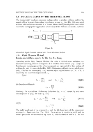
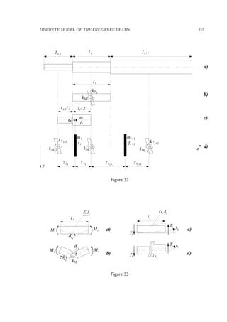
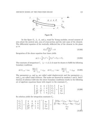
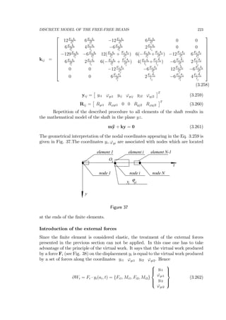
![DISCRETE MODEL OF THE FREE-FREE BEAMS 219
After introduction of Eq. 3.237 into the equation of the deflected line 3.234 one may
get it in the following form.
y(z) =
"
1 − 3
µ
z
li
¶2
+ 2
µ
z
li
¶3
#
yi1 +
"µ
z
li
− 2
µ
z
li
¶2
+
µ
z
li
¶3
#
liϕyi1
+
"
3
µ
z
li
¶2
− 2
µ
z
li
¶3
#
yi2 +
"
−
µ
z
li
¶2
+
µ
z
li
¶3
#
liϕyi2
= {H(z)}T
{y} (3.238)
where:
{H(z)} =
⎧
⎪⎪⎨
⎪⎪⎩
H1
H2li
H3
H4li
⎫
⎪⎪⎬
⎪⎪⎭
=
⎧
⎪⎪⎪⎪⎪⎪⎪⎪⎨
⎪⎪⎪⎪⎪⎪⎪⎪⎩
1 − 3
³
z
li
´2
+ 2
³
z
li
´3
∙³
z
li
´
− 2
³
z
li
´2
+
³
z
li
´3
¸
li
3
³
z
li
´2
− 2
³
z
li
´3
∙
−
³
z
li
´2
+
³
z
li
´3
¸
li
⎫
⎪⎪⎪⎪⎪⎪⎪⎪⎬
⎪⎪⎪⎪⎪⎪⎪⎪⎭
(3.239)
{y} =
⎧
⎪⎪⎨
⎪⎪⎩
yi1
ϕyi1
yi2
ϕyi2
⎫
⎪⎪⎬
⎪⎪⎭
(3.240)
Functions H1, H2, H3, H4 (see Eq. 3.239) are known as Hermite cubics or shape func-
tions. The matrix {y} contains the nodal coordinates. As it can be seen from Eq.
3.238 the deflected line of the finite element is assembled of terms which are linear
with respect to the nodal coordinates.
If the finite element performs motion with respect to the stationary system of
coordinates xyz, it is assumed that the motion in the plane yz can be approximated
by the following equation.
y(z, t) = {H(z)}T
{y (t)} (3.241)
As one can see from the equation 3.241, the dynamic deflection line is approximated
by the static deflection line. It should be noted that this assumption is acceptable
only if the considered element is reasonably short.
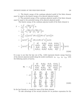
The following mathematical manipulations are aimed to replace the continues
mathematical model of the element considered
EiJi
∂4
y(z, t)
∂z4
− ρi
∂2
y(z, t)
∂t2
= 0 (3.242)
by its discreet representation along the nodal coordinates
[mi] {¨y (t)} + [ki] {y (t)} = 0. (3.243)
In the above equations ρi stands for the unit mass of the finite element and [mi] and
[ki] stands for the inertia and stiffness matrix respectively. These two matrices are
going to be developed from the two following criterions:](https://image.slidesharecdn.com/mechanicalvibrationbyjanuszkrodkiewski-130817083717-phpapp01/85/Mechanical-vibration-by-janusz-krodkiewski-219-320.jpg)
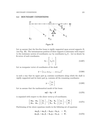
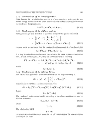
![CONDENSATION OF THE DISCREET SYSTEMS 227
To eliminate the coordinates ye from the mathematical model 3.279, one have to
determine the relationship between the coordinates ye and the coordinates yr. One
of many possibilities is to assume that the coordinates ye are obeyed to the static
relationship. ∙
kee ker
kre krr
¸ ∙
ye
yr
¸
=
∙
0
0
¸
(3.280)
Hence, upon partitioning equation 3.280 one may obtain
keeye+keryr= 0 (3.281)
Therefore the sought relationship is
ye= hyr (3.282)
where
h = −k−1
ee ker (3.283)
Once the relationship is established, one may formulate the following criteria of con-
densation:
1. Kinetic energy of the system before and after condensation must be the
same.
2. Dissipation function of the system before and after condensation must be
the same.
3. Potential energy of the system before and after condensation must be the
same.
4. Virtual work done by all the external forces before and after condensation
must be the same.
3.5.1 Condensation of the inertia matrix.
According to the first criterion, the kinetic energy of the system before and after
condensation must be the same. The kinetic energy of the system before condensation
is
T =
1
2
£
˙yT
e ˙yT
r
¤
∙
mee mer
mre mrr
¸ ∙
˙ye
˙yr
¸
=
1
2
¡
˙yT
e mee ˙ye + ˙yT
e mer ˙yr + ˙yT
r mre ˙ye + ˙yT
r mrr ˙yr
¢
(3.284)
Introduction of 3.282 yields
T =
1
2
³
[h˙yr]T
meeh˙yr + [h˙yr]T
mer ˙yr + ˙yT
r mreh˙yr+˙yT
r mrr ˙yr
´
=
1
2
¡
˙yT
r hT
meeh˙yr+˙yT
r hT
mer ˙yr+˙yT
r mreh˙yr+˙yT
r mrr ˙yr
¢
=
1
2
¡
˙yT
r
£
hT
meeh + hT
mer+mreh + mrr
¤
˙yr
¢
(3.285)
Hence, if the kinetic energy after condensation is to be the same, the inertia matrix
after condensation mc must be equal to
mc= hT
meeh + hT
mer+mreh + mrr (3.286)](https://image.slidesharecdn.com/mechanicalvibrationbyjanuszkrodkiewski-130817083717-phpapp01/85/Mechanical-vibration-by-janusz-krodkiewski-227-320.jpg)
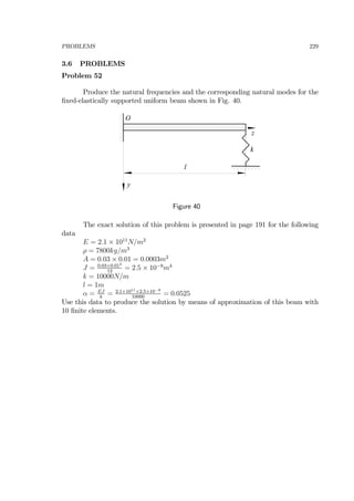
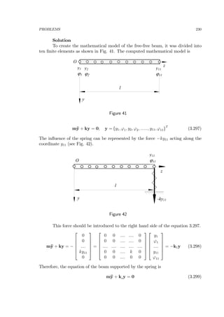
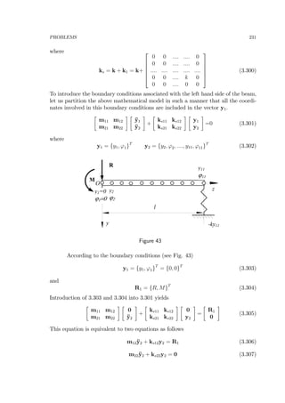
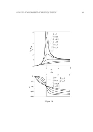
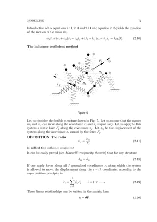
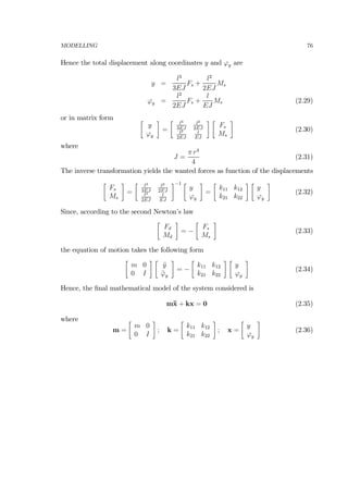
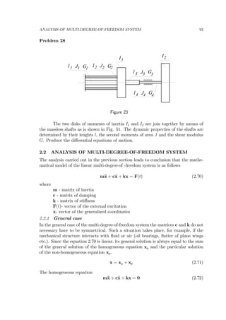
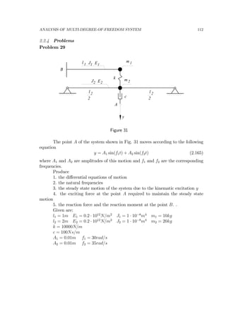
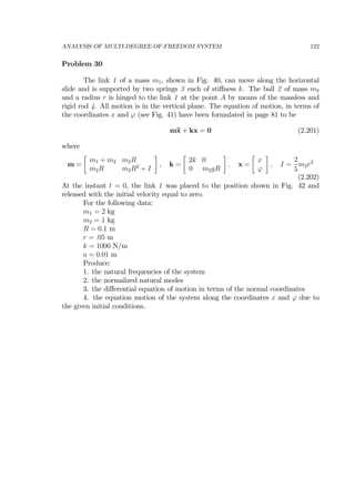
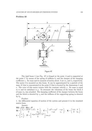
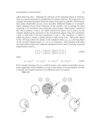
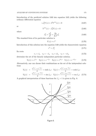
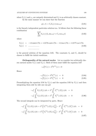
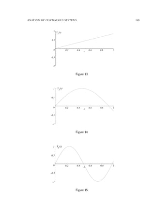
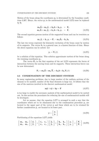
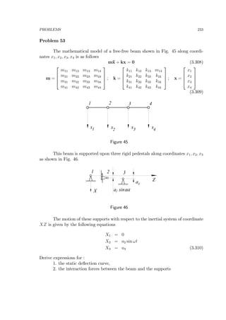
![PROBLEMS 232
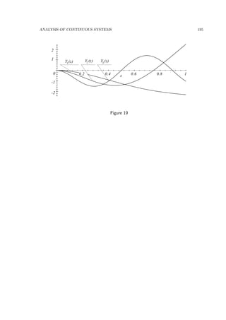
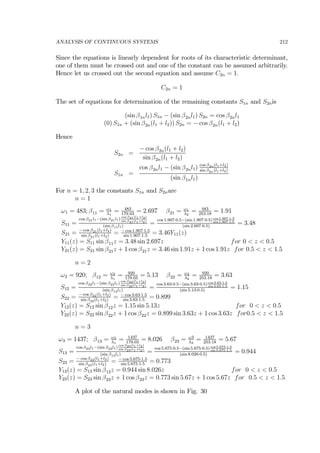
The second equation 3.307 is the equation of motion of the supported beam. It was
solved for the natural modes and the natural frequencies. Results of this computation
is shown in Fig. 44 by boxes and in the first column of the Table below. This results
are compare with natural modes (continuous line in Fig. 44) and natural frequencies
(second column in the Table) obtained by solving the continuous mathematical model
( see problem page 190). The equation 3.306 allows the vector of the interation forces
R1 to be computed.
-2
-1
0
1
2
0.2 0.4 0.6 0.8 1
z
Y1(z)
z
l k
y
O
Y3(z)Y2(z)
Figure 44
Table
natural frequenciesof
the descreet system
[1/sec]
natural frequencies of
the continuous system
[1/sec]
1 129.5 129.65
2 357.6 357.3
3 933.4 932.0](https://image.slidesharecdn.com/mechanicalvibrationbyjanuszkrodkiewski-130817083717-phpapp01/85/Mechanical-vibration-by-janusz-krodkiewski-232-320.jpg)
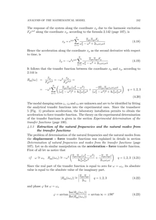
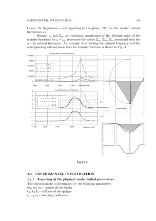
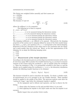
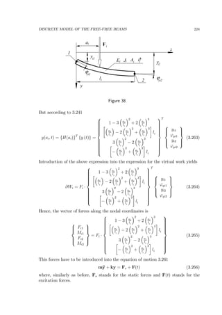
![ANALYSIS OF THE MATHEMATICAL MODEL 241
These equations can be rewritten as following
m¨x + c˙x + kx = F (4.9)
where
m =
⎡
⎣
m1 0 0
0 m2 0
0 0 m3
⎤
⎦ ; c =
⎡
⎣
c1 + c2 −c2 0
−c2 c2 + c3 −c3
0 −c3 c3
⎤
⎦
k =
⎡
⎣
k1 + k2 −k2 0
−k2 k2 + k3 −k3
0 −k3 k3
⎤
⎦ ; x =
⎡
⎣
x1
x2
x3
⎤
⎦ ; F =
⎡
⎣
F1
F2
F3
⎤
⎦ (4.10)
The vector F represents the external excitation that can be applied to the system.
4.3 ANALYSIS OF THE MATHEMATICAL MODEL
4.3.1 Natural frequencies and natural modes of the undamped system.
The matrix of inertia and the matrix of stiffness can be assessed from the dimensions
of the object. Hence, the natural frequencies and the corresponding natural modes
of the undamped system can be produced. Implementation of the particular solution
x = X cos ωt (4.11)
into the equation of the free motion of the undamped system
m¨x + kx = F (4.12)
results in a set of the algebraic equations that are linear with respect to the vector
X. ¡
−ω2
m + k
¢
X = 0 (4.13)
Solution of the eigenvalue and eigenvector problem yields the natural frequencies and
the corresponding natural modes.
±ω1, ±ω2, ±ω3 (4.14)
Ξ = [Ξ1, Ξ2, Ξ2] (4.15)
For detailed explanation see pages 102 to 105
4.3.2 Equations of motion in terms of the normal coordinates - transfer
functions
If one assume that the damping matrix is of the following form
c =µm+κk (4.16)
the equations of motion 4.9 can be expressed in terms of the normal coordinates
η = Ξ−1
x (see section normal coordinates - modal damping page 105)
¨ηn + 2ξnωn ˙ηn + ω2
nηn = ΞT
n F(t), n = 1, 2, 3 (4.17)](https://image.slidesharecdn.com/mechanicalvibrationbyjanuszkrodkiewski-130817083717-phpapp01/85/Mechanical-vibration-by-janusz-krodkiewski-241-320.jpg)