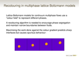
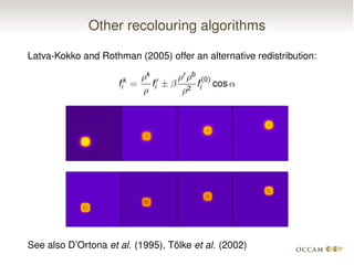
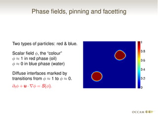
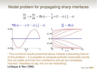
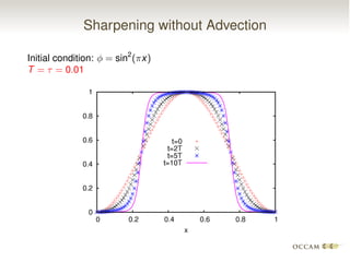
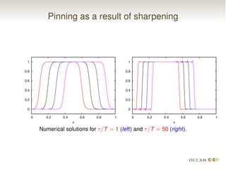
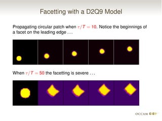
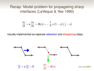
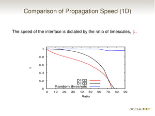
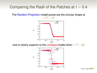
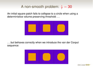
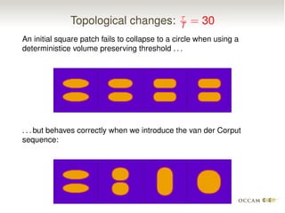
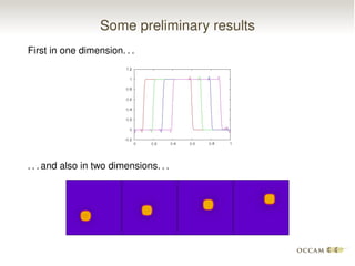
The document discusses issues with pinning and facetting in lattice Boltzmann simulations of multiphase flows. It presents a lattice Boltzmann model for propagating sharp interfaces using a phase field approach. Sharpening the phase field interface causes it to become pinned to the lattice or develop facets. Introducing randomness via a random projection method or random threshold prevents pinning and delays facetting, allowing the interface to propagate at the correct speed even for very sharp boundaries.

1. Pinning and facetting in lattice Boltzmann
simulations
Tim Reis
Oxford Centre for Collaborative Applied Mathematics
Mathematical Institute
University of Oxford
OCCAM/ICFD Lattice Boltzmann Workshop, September
2010

2. Recolouring in multiphase lattice Boltzmann models
Lattice Boltzmann models for continuum multiphase flows use a
“colour field" to represent different phases.
A recolouring algorithm is needed to encourage phase segregation
and maintain narrow boundaries between fluids.
Maximising the work done against the colour gradient predicts sharp
interfaces but causes spurious behaviour:

3. Other recolouring algorithms
Latva-Kokko and Rothman (2005) offer an alternative redistribution:
fk
i =
⇢k
⇢
f0
i ±
⇢r
⇢b
⇢2
f
(0)
i cos ↵
See also D’Ortona et al. (1995), Tölke et al. (2002)

4. Motivation
• Multiphase LBEs are prone to lattice pinning and facetting
(Latva-Kokko & Rothman (2005), Halliday et al. (2006)).
• Similar difficulties arise in combustion (Colella (1986), Pember
(1993)).
• Spurious phenomena associated with stiff source terms
investigated by LeVeque & Yee (1990).
• Unphysical behaviour can be corrected with a random projection
method (Bao & Jin (2000)).
• LB formulation of these models can shed light on pinning and
facetting.

5. Phase fields, pinning and facetting
Two types of particles: red & blue.
Scalar field , the “colour”
⇡ 1 in red phase (oil)
⇡ 0 in blue phase (water)
Diffuse interfaces marked by
transitions from ⇡ 1 to ⇡ 0.
@t + u · r = S( ).

6. Model problem for propagating sharp interfaces
@
@t
+ u
@
@x
= S( ) =
1
T
1 1
2
TS( ) = 1 1
2
d
dt = S( )
“ The numerical results presented above indicate a disturbing feature
of this problem – it is possible to compute perfectly reasonable results
that are stable and free from oscillations and yet are completely
incorrect. Needless to say, this can be misleading.”
LeVeque & Yee (1990)

7. Lattice Boltzmann Implementation
Suppose =
P
i fi and postulate the discrete Boltzmann equation:
@t fi + ci @x fi =
1
⌧
⇣
fi f
(0)
i
⌘
+ Ri .
With the following equilibrium function and discrete source term :
f
(0)
i = Wi (1 + ci u),
Ri = 1
2 S( )(1 + ci u);
the Chapman-Enskog expansion yields the
advection-reaction-diffusion equation:
@
@t
+ u
@
@x
= S( ) + ⌧(1 u2
)
@2
@x2
.

8. Reduction to Fully Discrete Form
The previous discrete Boltzmann equation can be written as
@t fi + ci @x fi = ⌦i
Integrate along a characteristic for time t:
fi (x + ci t, t + t) fi (x, t) =
Z t
0
⌦i (x + ci s, t + s) ds,
and approximate the integral by the trapezium rule:
fi (x +ci t, t+ t) fi (x, t) =
t
2
⇣
⌦i (x +ci t, t+ t)
+ ⌦i (x, t)
⌘
+O t3
.
This is an implicit system.

9. Change of Variables
To obtain a second order explicit LBE at time t + t define
fi (x0
, t0
) = fi (x0
, t0
)
t
2⌧
⇣
fi (x0
, t) f
(0)
i (x0
, t)
⌘ t
2
Ri (x0
, t)
The new algorithm is
fi (x + ci t , t + t) fi (x, t)
=
t
⌧ + t/2
⇣
fi (x, t) f
(0)
i (x, t)
⌘
+
⌧ t
⌧ + t/2
Ri (x, t),
However, we need to find in order to compute f
(0)
i and Ri .

10. Reconstruction of
The source term does not conserve :
¯ =
X
i
fi =
X
i

fi
t
2⌧
⇣
fi f
(0)
i
⌘ t
2
Ri
= +
t
2T
1 1
2 = N( ).
We can reconstruct by solving the nonlinear equation N( ) = ¯
using Newton’s method:
!
N( ) ¯
N0( )
,
Note that N( ) = + O( t/T).

11. Lengthscale of Transition
The diffusive extension of LeVeque and Yee’s model is
@
@t
+ u
@
@x
= S( ) + 
@2
@x2
Solving the ODE
0 = S( ) + 
@2
@x2
gives us the interface profile
(x) = (1 + exp x/L)
1
,
where L =
p
2⌧T x is the lengthscale of transition

12. Sharpening without Advection
Initial condition: = sin2
(⇡x)
T = ⌧ = 0.01

13. Pinning as a result of sharpening
Numerical solutions for ⌧/T = 1 (left) and ⌧/T = 50 (right).

14. Conservation Trouble
In the 2D case the circular region shrinks and eventually disappears:
This is due to the curvature of the interface:
We find c that satisfies
M =
Z
⌦
S( , c)d⌦.

15. Facetting with a D2Q9 Model
Propagating circular patch when ⌧/T = 10. Notice the beginnings of
a facet on the leading edge . . .
When ⌧/T = 50 the facetting is severe . . .

16. Recap: Model problem for propagating sharp
interfaces (LeVeque & Yee 1990)
@
@t
+ u
@
@x
= S( ) =
1
T
1 1
2
Usually implemented as separate advection and sharpening steps.
@
@t + u @
@x = 0
@
@t
= S( )

17. The Random Projection Method
The LeVeque & Yee source term is effectively the deterministic
projection
SD( ) : (x, t + t) =
(
1 if 0
(x, t) > 1/2,
0 if 0
(x, t)  1/2.
Bao & Jin (2000) replace the critical c = 1/2 with a uniformly
distributed random variable
(n)
c :
SR( ) : (x, t + t) =
(
1 if 0
(x, t) >
(n)
c ,
0 if 0
(x, t) 
(n)
c .
@
@t
+ u · r =
1
T
1 (n)
c .

18. Comparison of Propagation Speed (1D)
The speed of the interface is dictated by the ratio of timescales, ⌧
T .

19. Comparing the Radii of the Patches at t = 0.4
The Random Projection model preserves the circular shape at
⌧/T = 10
and is clearly superior to the LeVeque model when ⌧/T = 30

20. A non-smooth problem: ⌧
T = 30
An initial square patch fails to collapse to a circle when using a
deterministice volume preserving threshold . . .
. . . but behaves correctly when we introduce the van der Corput
sequence:

21. Topological changes: ⌧
T = 30
An initial square patch fails to collapse to a circle when using a
deterministice volume preserving threshold . . .
. . . but behaves correctly when we introduce the van der Corput
sequence:

22. A conservative scheme
If we assume L =
p
2⌧T x then
@
@n
= r · n = |r | =
(1 )
L
,
@2
@n2
=
(r · r)|r |
|r |
=
(1 )(1
2 )
L2
.
We can now show that a DBE of the form
@fi
@t
+ ci
@fi
@x
=
1
⌧
⇣
fi f
(0)
i
⌘
+ Wi
(1 )
L
ci · n
furnishes
@
@t
+ u
@
@x
= ⌧(1 u2
)r2
+ ⌧r2 (1 )(1
2 )
T
in the macroscopic limit.

23. Some preliminary results
First in one dimension. . .
. . . and also in two dimensions. . .

24. Conclusion
• We have studied the combination of advection and sharpening of
the phase field that commonly arises in lattice Boltzmann models
for multiphase flows.
• Overly sharp phase boundaries can become pinned to the
lattice. This has been shown to be a purely kinematic effect.
• Replacing the threshold with a uniformly distributed
pseudo-random variable allows us to predict the correct
propagation speed at very sharp boundaries (⌧/T > 100).
• The onset of facetting is signifficanly delayed if we introduce a
random term into the volume-preserving multi-dimensional
extension.