
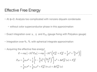
![On the Starting Line: Lattice QCD
• 1 flavor staggered fermion (4 flavor in continuum limit), color SU(3)
• Detail of action
Z =
Z
D [U0, Uj, , ¯] exp
"
S
(⌧)
F S
(s)
F
X
x
m0 ¯a
x
a
x SG
#
S
(⌧)
F =
1
2
X
x
h
eµ
¯xU0,x x+ˆ0 e µ
¯x+ˆ0U†
0,x x
i
S
(s)
F =
1
2
X
x,j
⌘j,x
h
¯xUj,x x+ˆj ¯x+ˆjU†
j,x x
i
⌘j,x = ( 1)
x0+x1+···xj 1
(j = 1, 2, 3) .
SG =
2Nc
g2
1
trc
2Nc
⇥
Uµ⌫,x + U†
µ⌫,x
⇤
! 0 g2
! 1
Strong coupling limit](https://image.slidesharecdn.com/masterbenjaminfinaliii-141103175140-conversion-gate01/85/Phase-diagram-at-finite-T-Mu-in-strong-coupling-limit-of-lattice-QCD-4-320.jpg)

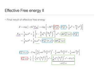
![Introduction
• Analytical approach (Kawamoto et al. ’07)
• 1 flavor staggered fermion (4 flavor in continuum limit), color SU(3)
• Detail of action
Z =
Z
D [U0, Uj, , ¯] exp
"
S
(⌧)
F S
(s)
F
X
x
m0 ¯a
x
a
x SG
#
Strong coupling limit
a⌧ = as = 1
S
(⌧)
F = a3
sa⌧
X
x
"
eµa⌧
¯xU0,x x+ˆ0 e µa⌧
¯x+ˆ0U†
0,x x
2a⌧
#
S
(s)
F = a3
sa⌧
X
x,j
⌘j,x
"
¯xUj,x x+ˆj ¯x+ˆjU†
j,x x
2as
#
⌘j,x = ( 1)
x0+x1+···xj 1
(j = 1, 2, 3) .
SG =
2Nc
g2
1
trc
2Nc
⇥
Uµ⌫,x + U†
µ⌫,x
⇤
! 0 g2
! 1](https://image.slidesharecdn.com/masterbenjaminfinaliii-141103175140-conversion-gate01/85/Phase-diagram-at-finite-T-Mu-in-strong-coupling-limit-of-lattice-QCD-6-320.jpg)
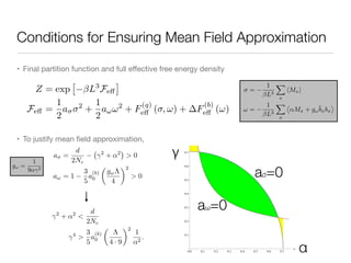
![SU(3) Group Integral with Spatial Link Variable
• Kluberg-Stern et al. (’83)
Mx = ¯a
x
a
x
Bx =
1
Nc!
"a1a2···aNc a1 a2
· · · aNc
¯Bx =
1
Nc!
"a1a2···aNc
¯aNc
· · · ¯a2
¯a1
Z
D [Uj] e S
(s)
F =
Z
D [Uj] exp
2
4 1
2
·
X
x,j
⌘j,x
⇣
¯xUj,x x+ˆj ¯x+ˆjU†
j,x x
⌘
3
5
= exp
2
4
X
x
1
4Nc
dX
j=1
MxMx+ˆj
X
x
( 1)
Nc(Nc 1)
2
dX
j=1
⇣⌘j,x
2
⌘Nc
h
¯BxBx+ˆj + ( 1)
Nc ¯Bx+ˆjBx
i
X
x
N2
c · (Nc 2)! Nc!
32 · N2
c · Nc!
dX
j=1
M2
xM2
x+ˆj
X
x
2 · Nc! N3
c · (Nc 2)!
128 · N4
c · Nc!
dX
j=1
M3
xM3
x+ˆj
3
5](https://image.slidesharecdn.com/masterbenjaminfinaliii-141103175140-conversion-gate01/85/Phase-diagram-at-finite-T-Mu-in-strong-coupling-limit-of-lattice-QCD-7-320.jpg)
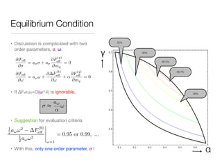
![Systematic 1/d Expansion I
• At d (space dimension) →∞, mean field theory becomes exact.
• demand the leading order term be O(1) at d→∞ : Rescale quark field
x ! d
1
4
x
Mx =
p
d · [¯a
x
a
x]
Bx = d
Nc
4 ·
1
Nc!
"a1a2···aNc a1 a2
· · · aNc
¯Bx = d
Nc
4 ·
1
Nc!
"a1a2···aNc
¯aNc
· · · ¯a2
¯a1](https://image.slidesharecdn.com/masterbenjaminfinaliii-141103175140-conversion-gate01/85/Phase-diagram-at-finite-T-Mu-in-strong-coupling-limit-of-lattice-QCD-8-320.jpg)
![Systematic 1/d Expansion II
• Then our result looks like
• Kluberg-Stern et al. (’83) : Contribution of higher order terms to Vacuum Expectation Value of chiral
condensate(<ψψ>) is small at zero temperature(T=0). (In d=4, about 7%)
• Usually, Analyzed only in O(1): Damgaard et al.(’84), Nishida(’04), Miura et al.(’07), Nakano et al.(’10),... etc.
• We want to investigate the baryon effect: We adopt not only O(1) but also O(1/√d) for our effective action.
Z
D [Uj] e S
(s)
F = exp
2
4
X
x
1
d
dX
j=1
⇢
1 ·
✓
1
4Nc
· MxMx+ˆj
◆
+
1
p
dNc 2
·
✓
( 1)
Nc(Nc 1)
2
⇣⌘j,x
2
⌘Nc
·
⇣
¯BxBx+ˆj + ( 1)
Nc ¯Bx+ˆjBx
⌘◆
+
1
d
·
✓
N2
c · (Nc 2)! Nc!
32 · N2
c · Nc!
· M2
xM2
x+ˆj
◆
+
1
d2
·
✓
2 · Nc! N3
c · (Nc 2)!
128 · N4
c · Nc!
· M3
xM3
x+ˆj
◆
O(1)
O(1/√d) @ Nc=3
O(1/d)
O(1/d^2)](https://image.slidesharecdn.com/masterbenjaminfinaliii-141103175140-conversion-gate01/85/Phase-diagram-at-finite-T-Mu-in-strong-coupling-limit-of-lattice-QCD-9-320.jpg)
![After the Path Integral of Spatial Link Variable
• So far, our partition function
• Propagators and inner product
VM,xy =
1
2d
dX
j=1
⇣
y,x+ˆj + y,x ˆj
⌘
VB,xy = ( 1)
Nc(Nc 1)
2
dX
j=1
⇣⌘j,x
2
⌘Nc
⇣
y,x+ˆj + ( 1)
Nc
y,x ˆj
⌘
(A, V B) =
X
x,y
AxVxyBy
Z =
Z
D [U0, Uj, , ¯] exp
"
S
(⌧)
F
X
x
m0 ¯a
x
a
x S
(s)
F
#
⇡
Z
D [U0, , ¯] exp
"
S
(⌧)
F
X
x
m0Mx +
d
2Nc
·
1
2
(M, VM M) + ¯B, VBB
#](https://image.slidesharecdn.com/masterbenjaminfinaliii-141103175140-conversion-gate01/85/Phase-diagram-at-finite-T-Mu-in-strong-coupling-limit-of-lattice-QCD-10-320.jpg)
![Bosonization: Introducing Auxiliary Fields
• We want the bilinear form of quark → Hubbard-Stratonovich transformation
Da;x =
2
"abc
b
x
c
x +
1
3
¯a
xbx
D†
a;x =
2
"abc ¯c
x ¯b
x +
1
3
¯bx
a
x
d
2Nc
·
1
2
(M, VM M)
2
2
(M, M)
↵2
2
(M, M) =
1
2
⇣
M, eVM M
⌘
¯b, V 1
B b g!! ¯b, b =
⇣
¯b, eV 1
B b
⌘
e( ¯B,VBB) = det VB
Z
D
⇥
¯b, b
⇤
e (¯b,V 1
B b)+(¯b,B)+( ¯B,b)
e( ¯B,b)+(¯b,B) =
Z
d
⇥
a, †
a
⇤
exp
"
†
a, a +
X
x
†
a;xDa;x + D†
a;x a;x
2
2
(M, M) +
X
x
1
9 2
Mx
¯bxbx
#
e
P
x
1
9 2 Mx
¯bxbx
=
Z
D [!] exp
"
1
2
(!, !) ↵
X
x
Mx + g!
¯bxbx !x
↵2
2
(M, M)
#
e
1
2 (M,eVM M) =
Z
D [ ] exp
1
2
⇣
, eVM
⌘ ⇣
, eVM M
⌘
Z =
Z
D [U0, , ¯] exp
"
S
(⌧)
F +
d
2Nc
·
1
2
(M, VM M) + ¯B, VBB
X
x
m0Mx
#
g! =
1
9↵ 2
free parameters α, γ](https://image.slidesharecdn.com/masterbenjaminfinaliii-141103175140-conversion-gate01/85/Phase-diagram-at-finite-T-Mu-in-strong-coupling-limit-of-lattice-QCD-11-320.jpg)


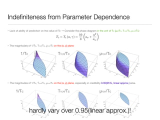


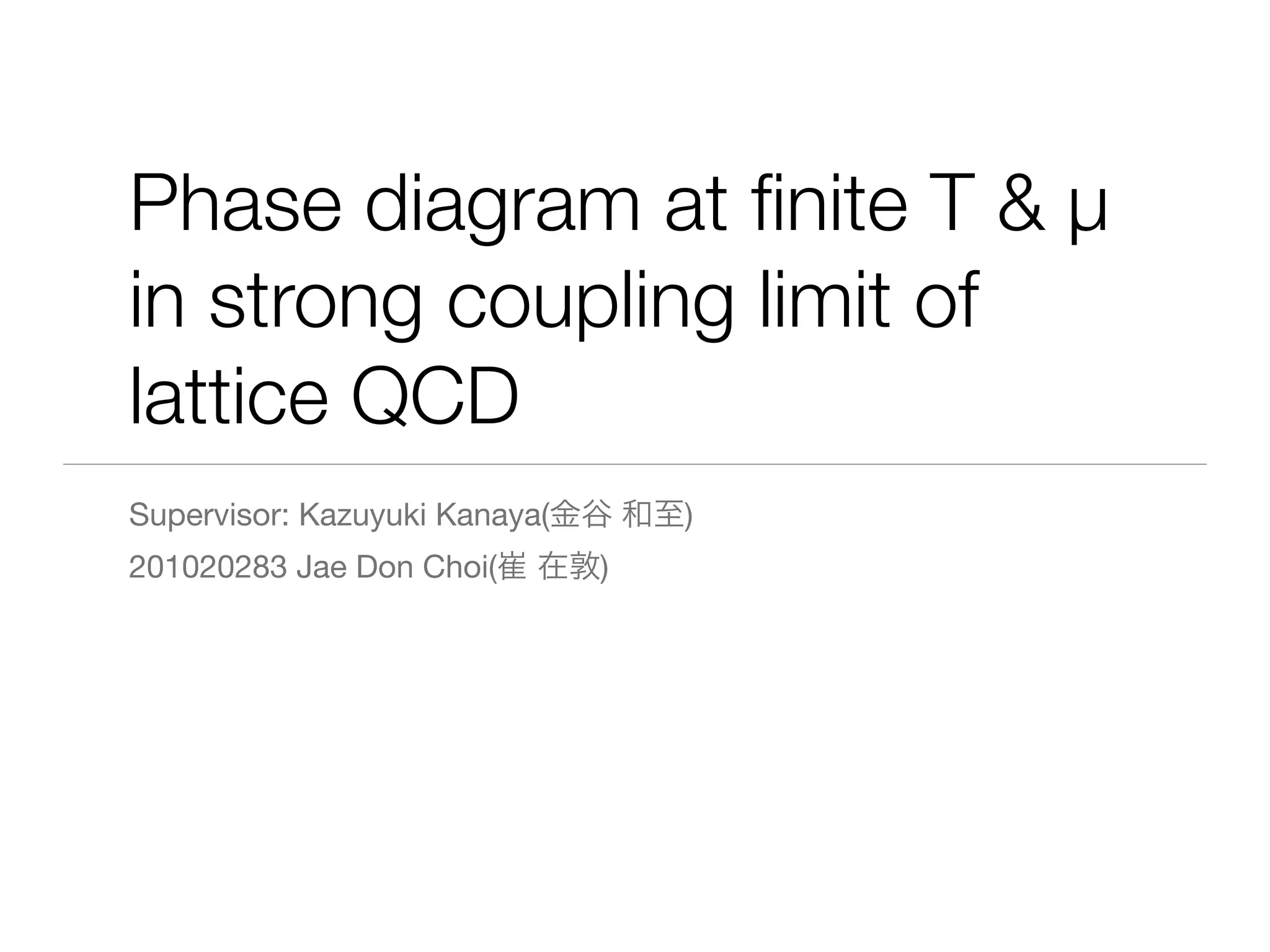
This document summarizes the derivation of an effective free energy for QCD at strong coupling using a mean field approximation with 1 flavor staggered fermion. Key steps include: 1) Performing a path integral over spatial link variables to obtain quark propagators. 2) Introducing auxiliary bosonic fields using a Hubbard-Stratonovich transformation to obtain a bilinear form in quark fields. 3) Applying a mean field approximation to the auxiliary fields. 4) Exactly integrating over temporal links, quark and auxiliary baryon fields to obtain an effective free energy in terms of the auxiliary meson field. 5) Analyzing the effective free energy to determine the QCD phase diagram as functions of temperature and


![Mathematics of nyquist plot [autosaved] [autosaved]](https://cdn.slidesharecdn.com/ss_thumbnails/mathematicsofnyquistplotautosavedautosaved-150219123133-conversion-gate02-thumbnail.jpg?width=640&height=640&fit=bounds)


![Polymer [ बहुलक ] Chemistry Notes PDF - Irfanullah Mehar - JJ Sir Chemistry.pdf](https://cdn.slidesharecdn.com/ss_thumbnails/polymerchemistrynotespdf-irfanullahmehar-jjsirchemistry-260210172118-3f9b37f7-thumbnail.jpg?width=640&height=640&fit=bounds)


