Download as PDF, PPTX
![7
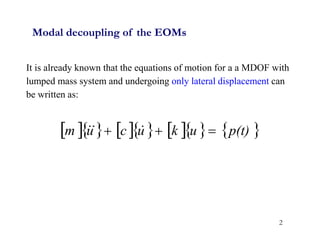
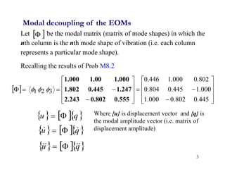
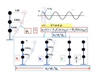
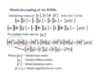
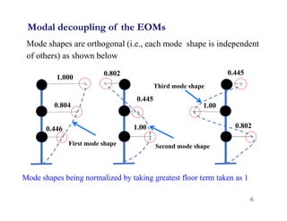
Modal decoupling of the EOMs
A matrix said to be orthogonal if where [I] is
an identity matrix in which diagonal terms are 1 and off diagonal
terms are 0 and therefore det [I]=1. are diagonal
matrices (i.e., matrices in which off diagonal terms are zero)
A
I
A
A
T
C
and
K
,
M
m1
m2
m3
k1
k2
k3
3
2
1
m
0
0
0
m
0
0
0
m
m
m3
m2
m1](https://image.slidesharecdn.com/module9-220516150605-a7ea8c03/85/Module-9-Spring-2020-pdf-7-320.jpg)
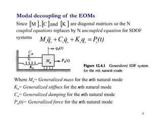
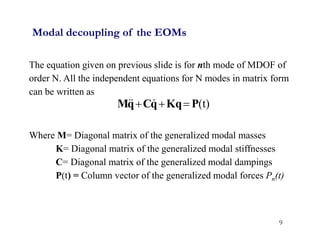
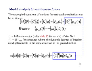
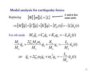
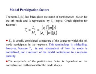
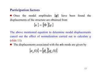
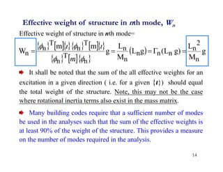
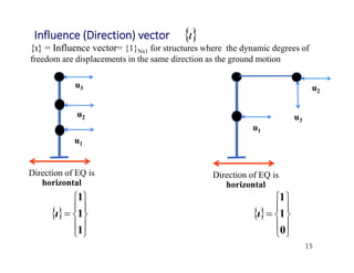
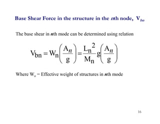
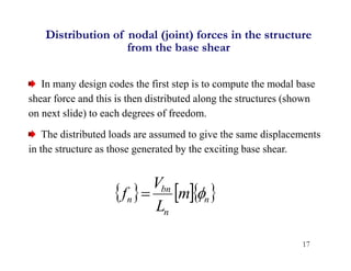
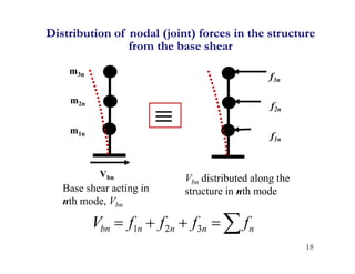
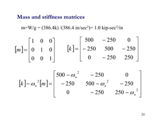
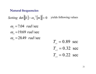
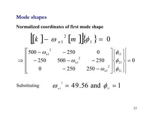
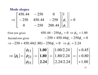
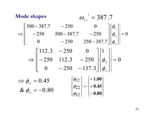
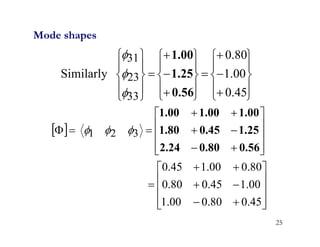
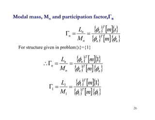
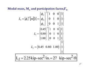
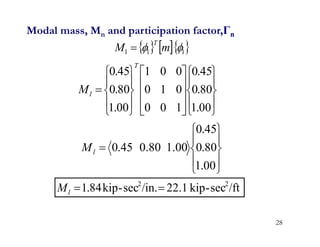
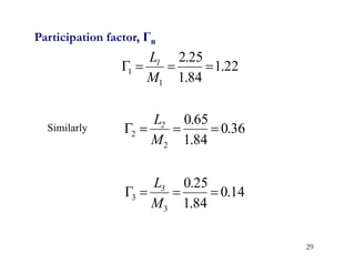
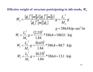
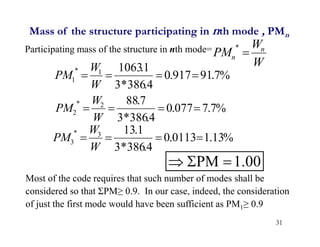
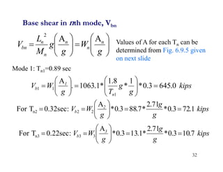
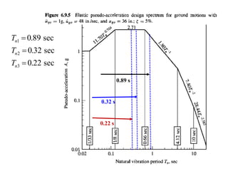
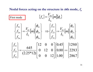
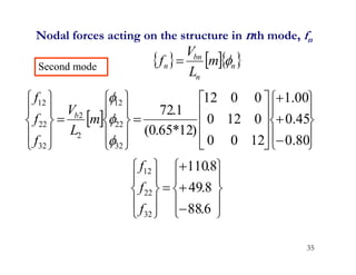
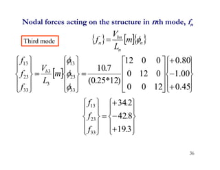
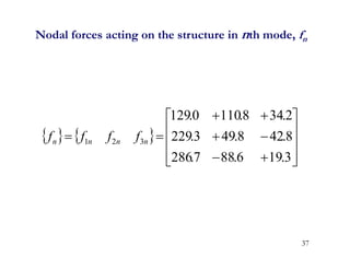
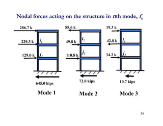
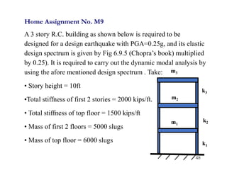

This document discusses modal response spectrum analysis for earthquake engineering. Some key points: - The equations of motion for a multi-degree of freedom structural system can be decoupled into individual single-degree of freedom equations through modal analysis. - Mode shapes are orthogonal and form a modal matrix that transforms displacement coordinates into modal coordinates. This results in uncoupled equations for each vibration mode. - Earthquake excitation is represented as a modal force vector. Response of each mode is then determined independently through its modal mass, stiffness and damping. - Participation factors relate the modal displacements back to the physical displacements of the structure and determine the effective modal weight contributing to response in each mode.


![Module 14 [Compatibility Mode].pdf](https://cdn.slidesharecdn.com/ss_thumbnails/module14compatibilitymode-221005020212-a4e2d1ee-thumbnail.jpg?width=640&height=640&fit=bounds)