Download as PDF, PPTX


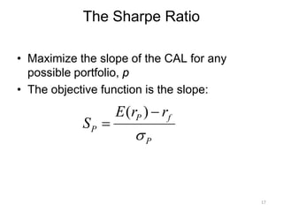
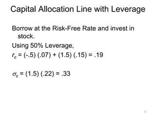
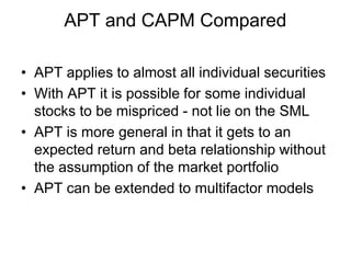
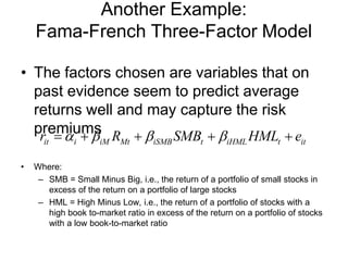
![CAPM results
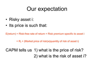
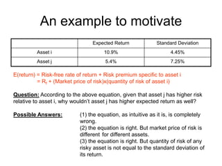
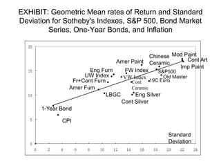
E(return) = Risk-free rate of return + Risk premium specific to asset i
= Rf + (Market price of risk)x(quantity of risk of asset i)
Precisely:
[1] Expected Return on asset i = E(Ri)
[2] Equilibrium Risk-free rate of return = Rf
[3] Quantity of risk of asset i = COV(Ri, RM)/Var(RM)
[4] Market Price of risk = [E(RM)-Rf]
Thus, the equation known as the Capital Asset Pricing Model:
E(Ri) = Rf + [E(RM)-Rf] x [COV(Ri, RM)/Var(RM)]
Where [COV(Ri, RM)/Var(RM)] is also known as BETA of asset I
Or
E(Ri) = Rf + [E(RM)-Rf] x βi](https://image.slidesharecdn.com/portfoliotheoryandcapm-150605200848-lva1-app6892/85/Portfolio-theory-and-capm-9-320.jpg)
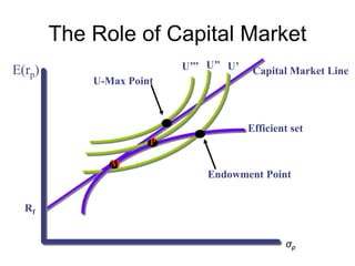
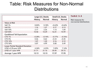
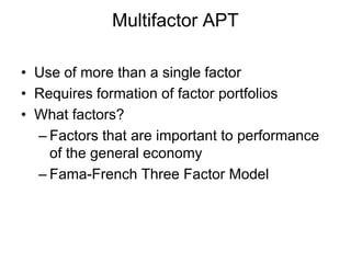
![Pictorial Result of CAPM
E(Ri)
E(RM)
Rf
Security
Market
Line
β =
[COV(Ri, RM)/Var(RM)]βΜ= 1.0
slope = [E(RM) - Rf] = Eqm. Price of risk](https://image.slidesharecdn.com/portfoliotheoryandcapm-150605200848-lva1-app6892/85/Portfolio-theory-and-capm-10-320.jpg)
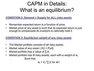
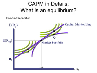
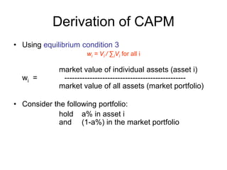
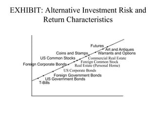
![CAPM in Details:
What is an equilibrium?
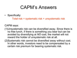
CONDITION 1: Individual investor’s equilibrium: Max U
• Assume:
• [1] Market is frictionless
=> borrowing rate = lending rate
=> linear efficient set in the return-risk space
[2] Anyone can borrow or lend unlimited amount at risk-free rate
• [3] All investors have homogenous beliefs
=> they perceive identical distribution of expected returns on
ALL assets
=> thus, they all perceive the SAME linear efficient set (we
called the line: CAPITAL MARKET LINE
=> the tangency point is the MARKET PORTFOLIO](https://image.slidesharecdn.com/portfoliotheoryandcapm-150605200848-lva1-app6892/85/Portfolio-theory-and-capm-11-320.jpg)
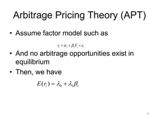
![CAPM
• 2 sets of Assumptions:
[1] Perfect market:
• Frictionless, and perfect information
• No imperfections like tax, regulations, restrictions to short
selling
• All assets are publicly traded and perfectly divisible
• Perfect competition – everyone is a price-taker
[2] Investors:
• Same one-period horizon
• Rational, and maximize expected utility over a mean-
variance space
• Homogenous beliefs](https://image.slidesharecdn.com/portfoliotheoryandcapm-150605200848-lva1-app6892/85/Portfolio-theory-and-capm-23-320.jpg)
![Derivation of CAPM
• The expected return and standard deviation of such a
portfolio can be written as:
E(Rp) = aE(Ri) + (1-a)E(Rm)
σ(Rp) = [ a2σi
2 + (1-a)2σm
2 + 2a (1-a) σim ] 1/2
• Since the market portfolio already contains asset i and,
most importantly, the equilibrium value weight is wi
• therefore, the percent a in the above equations represent
excess demands for a risky asset
• We know from equilibrium condition 2 that in equilibrium,
Demand = Supply for all asset.
• Therefore, a = 0 has to be true in equilibrium.](https://image.slidesharecdn.com/portfoliotheoryandcapm-150605200848-lva1-app6892/85/Portfolio-theory-and-capm-25-320.jpg)
![Derivation of CAPM
E(Rp) = aE(Ri) + (1-a)E(Rm)
σ(Rp) = [ a2σi
2 + (1-a)2σm
2 + 2a (1-a) σim ] 1/2
• Consider the change in the mean and standard deviation with
respect to the percentage change in the portfolio invested in
asset i
• Since a = 0 is an equilibrium for D = S, we must evaluate these
partial derivatives at a = 0
)RE(-)RE(=
a
)RE(
mi
p
∂
∂
]4a-2+2a+2-2a[*]a)-2a(1+)a-(1+a[
2
1
=
a
)R(
imim
2
m
2
m
2
i
1/2-
im
2
m
22
i
2p
σσσσσσσσ
σ
∂
∂
)RE(-)RE(=
a
)RE(
mi
p
∂
∂
σ
σσσ
m
2
mimp -
=
a
)R(
∂
∂
(evaluated at a = 0)
(evaluated at a = 0)](https://image.slidesharecdn.com/portfoliotheoryandcapm-150605200848-lva1-app6892/85/Portfolio-theory-and-capm-26-320.jpg)
![Derivation of CAPM
• the slope of the risk return trade-off evaluated at point M in
market equilibrium is
• but we know that the slope of the opportunity set at point M must
also equal the slope of the capital market line. The slope of the
capital market line is
• Therefore, setting the slope of the opportunity set equal to the
slope of the capital market line
• rearranging,
σ
σσσ
m
2
mim
mi
p
p
-
)RE(-)RE(
=
a)/R(
a)/RE(
∂∂
∂∂
σ m
fm R-)RE(
σσσσ m
fm
m
2
mim
mi R-)RE(
=
/)-(
)RE(-)RE(
]R-)R[E(+R=)RE( fm2
m
im
fi
σ
σ
(evaluated at a = 0)](https://image.slidesharecdn.com/portfoliotheoryandcapm-150605200848-lva1-app6892/85/Portfolio-theory-and-capm-27-320.jpg)
![Derivation of CAPM
• From previous page
• Rearranging
• Where
E(return) = Risk-free rate of return + Risk premium specific to asset i
E(Ri) = Rf + (Market price of risk)x(quantity of risk of asset i)
CAPM Equation
)RVAR(
)R,RCOV(
==
m
mi
2
m
im
i
σ
σβ
βifmfi ]R-)R[E(+R=)RE(
]R-)R[E(+R=)RE( fm2
m
im
fi
σ
σ](https://image.slidesharecdn.com/portfoliotheoryandcapm-150605200848-lva1-app6892/85/Portfolio-theory-and-capm-28-320.jpg)
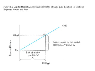
![CML Equation
• Y = b + mX
This leads to the Security Market Line (SML)
( )
[ ]FM
M
P
F
P
M
FM
FP
RRE
RSD
RSD
R
RSD
RSD
RRE
RRE
−+=
−
+=
)(
)(
)(
givesgrearrangin
)(
)(
)(](https://image.slidesharecdn.com/portfoliotheoryandcapm-150605200848-lva1-app6892/85/Portfolio-theory-and-capm-30-320.jpg)

![Pictorial Result of CAPM
E(Ri)
E(RM)
Rf
Security Market
Line
β =
[COV(Ri, RM)/Var(RM)]βΜ= 1.0
slope = [E(RM) - Rf] = Eqm. Price of risk](https://image.slidesharecdn.com/portfoliotheoryandcapm-150605200848-lva1-app6892/85/Portfolio-theory-and-capm-34-320.jpg)
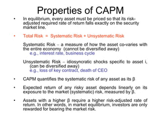
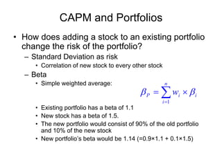


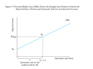
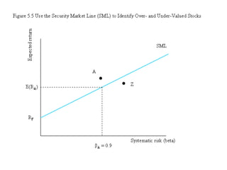
The document elaborates on portfolio theory and the Capital Asset Pricing Model (CAPM), detailing how assets are priced and the equilibrium conditions between individual investors and asset suppliers. It explains key concepts such as the risk-free asset, expected return, systematic vs. unsystematic risk, and the derivation of the CAPM equation linking expected returns to risk. Additionally, it discusses assumptions behind CAPM, the significance of beta, and the practical applications of this model in asset valuation and estimating required rates of return.


