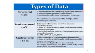
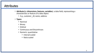
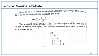
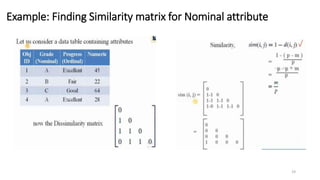
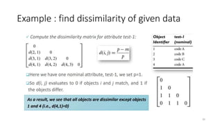
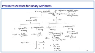
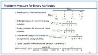
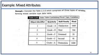
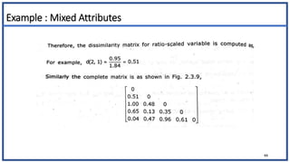
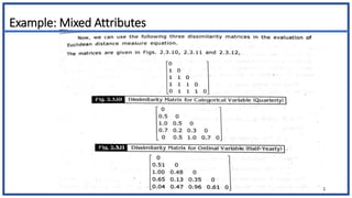
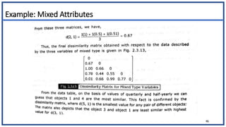
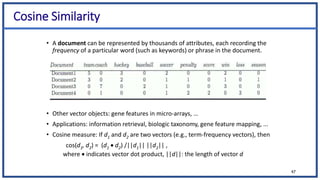
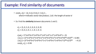
The document discusses various types of data sets and their attributes, categorizing them into structured, unstructured, semi-structured, and quasi-structured types. It also covers similarity and dissimilarity measures for data objects, including measures for nominal, binary, ordinal, and numeric attributes, while introducing concepts such as proximity measures and the cosine similarity formula. Additionally, it explains how to compute dissimilarity matrices using various distance metrics like Minkowski, and the importance of considering different attribute types in distance calculations.
![Proximity measure for Ordinal attributes
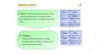
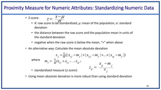
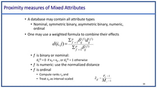
• An ordinal variable can be discrete or continuous
• Order is important, e.g., rank
• Can be treated like interval-scaled
• replace xif by their rank
• map the range of each variable onto [0, 1] by replacing i-th object in
the f-th variable by
• compute the dissimilarity using methods for interval-scaled variables
35
1
1
f
if
if M
r
z
}
,...,
1
{ f
if
M
r ](https://image.slidesharecdn.com/unit-iobjectsattributessimilaritydissimilarity-240509092520-a88f2b00/85/Unit-I-Objects-Attributes-Similarity-Dissimilarity-ppt-35-320.jpg)


![Wk. 3. Data [12-05-2021] (2).ppt](https://cdn.slidesharecdn.com/ss_thumbnails/wk-240205070901-8f81e253-thumbnail.jpg?width=640&height=640&fit=bounds)