Unit 3-Greedy Method

The general Method
 The greedy method is a most straight
forward design technique
 Most of these problems have n inputs and
require us to obtain a subset that satisfies
some constraints
 Any subset that satisfies the constraint is
called a feasible solution

 We need to find a feasible solution that
either maximizes or minimizes the given
objective function
 The Greedy method suggest an algorithm
that works in stages, considering one
input at a time
 At each stage a decision is made
regarding whether the particular input is
in an optimal solution

 This is done by selecting the input in a
particular order determined by some
selection procedure
 If the insertion of the next input into
partially constructed optimal solution will
result in an infeasible solution, then this
input is not added to the feasible solution.
Otherwise, it is added

 Algorithm Greedy(a,n)
{
solution:=¢;
For i:=1 to n do
{
X:= select(a);
If feasible(solution,x) then
Solution:=union(solution,x);
}
Return solution
}

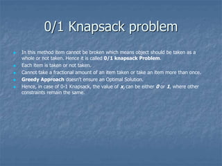
 The function select selects an input from
a[] and removes it .the selected input's
value is assigned to x. Feasible is a
Boolean valued function that determines
whether x can be included in to the
solution vector. The function union
combines x with the solution and updates
the objective function

Knapsack Problem
We are given n objects and a knapsack or a bag. Object i has a weight wi, and the
knapsack has a capacity m. If a fraction xi, 0<xi<1, of objects i is placed into the
knapsack, then a profit of pixi is earned.
The objective is to obtain a filling of the knapsack that maximizes the
total profit earned. Since the knapsack capacity is m, we require the total
weight of all chosen objects to be at most m. Formally the problem can
be stated as
The profits and weights are positive numbers.
A feasible solution (or filling) is any set (x1, x2,……,xn) satisfying
II and III above. An optimal solution is a feasible solution for which I is
maximized.

Exercise
1. Find an optimal solution to the knapsack instance n =4,
m=40,(p1,p2,p3,p4) = (20,40,35,45) and (w1,w2,w3,w4) = (20,25,10,15).
Strategy 1: consider the object in increasing order of weights
(w3,w4,w1,w2)
Remaining
capacity
object weight Fraction xi
included
40-10=30 3 10 1
30-15=15 4 15 1
15-15=0 1 20 15/20=3/4
Solution vector(x1,x2,x3,x4)=(3/4,0,1,1)
Profit=∑pixi=20*3/4+40*0+35*1+45*1=95

Strategy 2: consider the object in decreasing order of profit
(p4,p2,p3,p1)=(45,40,35,20)
Remaining
capacity
included
40-15=25 4 15 1
25-25=0 2 25 1
Solution vector(x1,x2,x3,x4)=(0,1,0,1)
Profit=∑pixi=20*0+40*1+35*0+45*1=85

Strategy 3: consider the object in decreasing order of profit/weight(pi/wi)
(P3/w3)>(p4/w4)>(p2/w2)>(p1/w1)
Remaining
capacity
included
40-10=30 3 10 1
30-15=15 4 15 1
15-15=0 2 25 15/25=3/5
Solution vector(x1,x2,x3,x4)=(0,3/4,1,1)
Profit=∑pixi=20*0+40*3/4+35*1+45*1=104

0/1 Knapsack problem
 In this method item cannot be broken which means object should be taken as a
whole or not taken. Hence it is called 0/1 knapsack Problem.
 Each item is taken or not taken.
 Cannot take a fractional amount of an item taken or take an item more than once.
 Greedy Approach doesn't ensure an Optimal Solution.
 Hence, in case of 0-1 Knapsack, the value of xi can be either 0 or 1, where other
constraints remain the same.

 Find an optimal solution to the knapsack instance n =4, m=40,(p1,p2,p3,p4) =
(20,40,35,45) and (w1,w2,w3,w4) = (20,25,10,15).
 Strategy 1: consider the object in increasing order of weights (w3,w4,w1,w2)
 Solution vector(x1,x2,x3,x4)=(0,0,1,1)
 Profit=∑pixi=20*0+40*0+35*1+45*1=80
 Even it the capacity of knapsack is not full, we do not consider the next object
i.e)object 1 .
Remaining
capacity
object weight Fraction of
xi
considered
40-10=30 3 10 1
30-15=15 4 15 1

 Strategy 2: consider the object in decreasing order of profits (p4,p3,p2,p1)
 Even it the capacity of knapsack is not full, we do not consider the next
object i.e)object 3 .
Profit=∑pixi=20*0+40*1+35*0+45*1=85
Remaining
capacity
xi
considered
40-15=25 4 15 1
25-25=0 2 25 1

 Strategy 3: consider the object in decreasing order of profits/weights
(p3/w3,p4/w4,p2/w2,p1/w1)
 Even it the capacity of knapsack is not full, we do not consider the
next object i.e)object 2 .
Profit=∑pixi=20*0+40*0+35*1+45*1=80
Remaining
capacity
xi
considered
40-10=30 3 10 1
30-15=15 4 15 1

MST – Minimum Spanning Tree
 Given a connected undirected graph we would like to
find the “cheapest” connected version of that graph
 Remove all extra edges leaving just enough to be
connected – it will be a tree
 A subgraph T=(V,E’)of G=(V,E) is a spanning tree if T is
a tree, and includes all vertices of G and subset of
edges(E’)
 Find the tree that has the smallest sum of edge lengths
 Given G = (V, E) and edge weights we, find the tree T =
(V, E') where E' ⊆ E and which also minimizes
is called Minimum Spanning Tree
 Not necessarily unique
 Many applications – cheapest phone network, etc.
CS 312 – Greedy Algorithms 17
we
eÎE'
å

Prims algorithm
 Prims algorithm constructs a minimum spanning tree
through sequence of expanding sub trees.
 It starts by selecting some arbitrary vertex V of graph of
vertices.
 On each iteration tree expands I greedy manner by
attaching nearest node not in the tree.
 Cost adjacency matrix gives the distance of present
vertex with all other vertices in the graph.
 If the vertex is not reachable from current vertex the
distance is given as ∞

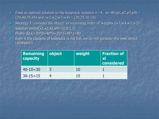
Prims algorithm
 //Assume that G is connected and weighted graph
 //Input: The cost adjacency matrix C and number of vertices n
 //Output: Minimum weight spanning tree T
Algorithm prims(c,n)
{
for i=1 to n do
visited[i]=0
u=1
Visited[u]=1
while there is still unchosen vertices do
{
let(u,v)be the lightest edge between any chosen u and v
Visited[v]=1
T’=union(T,<u,v>)
}
Return T
}

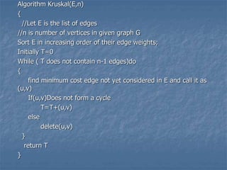
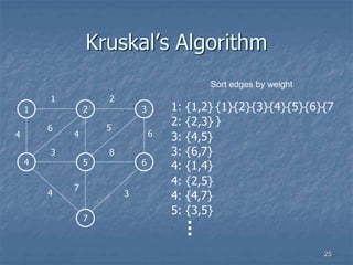
KRUSKAL'S ALGORITHM
This algorithm is used for finding the minimum cost
spanning tree for every connected undirected graph.
In the algorithm,
-> E is the set of edges in graph G
-> G has 'n' vertices
-> cost[u,v] is the cost of edge(u,v)
-> ‘T' is the set of edges in the minimum cost spanning
tree

Step1:Arrange the edges in increasing order of
weights
Step 2: Consider all vertices as independent
component
Step 3:Consider the edge if they belong to
different components and does not form a cycle,
reject otherwise.
Step 4: Repeat step 3 until single component
containing all vertices are included.

Algorithm Kruskal(E,n)
{
//Let E is the list of edges
//n is number of vertices in given graph G
Sort E in increasing order of their edge weights;
Initially T=0
While ( T does not contain n-1 edges)do
{
find minimum cost edge not yet considered in E and call it as
(u,v)
If(u,v)Does not form a cycle
T=T+(u,v)
else
delete(u,v)
}
return T
}

Kruskal’s Algorithm
1 2 3
1 2
4 5 6
3 8
7
4
6
4
5
6
7
3
4
{1}{2}{3}{4}{5}{6}{7
}
Make a disjoint set for each vertex
24

Sort edges by weight
1 2 3
1 2
4 5 6
3 8
7
4
6
4
5
6
7
3
4
1: {1,2}
2: {2,3}
3: {4,5}
3: {6,7}
4: {1,4}
4: {2,5}
4: {4,7}
5: {3,5}
{1}{2}{3}{4}{5}{6}{7
}
25

1 2 3
1 2
4 5 6
3 8
7
4
6
4
5
6
7
3
4
1: {1,2}
2: {2,3}
3: {4,5}
3: {6,7}
4: {1,4}
4: {2,5}
4: {4,7}
5: {3,5}
{1}{2}{3}{4}{5}{6}{7
}
Add first edge to X if no cycle created
26
CS 312 – Greedy Algorithms

1 2 3
1 2
4 5 6
3 8
7
4
6
4
5
6
7
3
4
1: {1,2}
2: {2,3}
3: {4,5}
3: {6,7}
4: {1,4}
4: {2,5}
4: {4,7}
5: {3,5}
{1,2}{3}{4}{5}{6}{7}
Merge vertices in added edges
27

1 2 3
1 2
4 5 6
3 8
7
4
6
4
5
6
7
3
4
1: {1,2}
2: {2,3}
3: {4,5}
3: {6,7}
4: {1,4}
4: {2,5}
4: {4,7}
5: {3,5}
{1,2}{3}{4}{5}{6}{7}
Process each edge in order
{1,2,3}{4}{5}{6}{7}
28

1 2 3
1 2
4 5 6
3 8
7
4
6
4
5
6
7
3
4
1: {1,2}
2: {2,3}
3: {4,5}
3: {6,7}
4: {1,4}
4: {2,5}
4: {4,7}
5: {3,5}
{1,2}{3}{4}{5}{6}{7}
{1,2,3}{4}{5}{6}{7}
{1,2,3}{4,5}{6}{7}
Note that each set is a connected component of G
29

1 2 3
1 2
4 5 6
3 8
7
4
6
4
5
6
7
3
4
1: {1,2}
2: {2,3}
3: {4,5}
3: {6,7}
4: {1,4}
4: {2,5}
4: {4,7}
5: {3,5}
{1,2}{3}{4}{5}{6}{7}
{1,2,3}{4}{5}{6}{7}
{1,2,3}{4,5}{6}{7}
{1,2,3}{4,5}{6,7}
30
CS 312 – Greedy Algorithms

1 2 3
1 2
4 5 6
3 8
7
4
6
4
5
6
7
3
4
1: {1,2}
2: {2,3}
3: {4,5}
3: {6,7}
4: {1,4}
4: {2,5}
4: {4,7}
5: {3,5}
{1,2}{3}{4}{5}{6}{7}
{1,2,3}{4}{5}{6}{7}
{1,2,3}{4,5}{6}{7}
{1,2,3}{4,5}{6,7}
{1,2,3,4,5}{6,7}
31

1 2 3
1 2
4 5 6
3 8
7
4
6
4
5
6
7
3
4
1: {1,2}
2: {2,3}
3: {4,5}
3: {6,7}
4: {1,4}
4: {2,5}
4: {4,7}
5: {3,5}
{1,2}{3}{4}{5}{6}{7}
Must join separate components
{1,2,3}{4}{5}{6}{7}
{1,2,3}{4,5}{6}{7}
{1,2,3}{4,5}{6,7}
{1,2,3,4,5}{6,7}
rejected
32

1 2 3
1 2
4 5 6
3 8
7
4
6
4
5
6
7
3
4
1: {1,2}
2: {2,3}
3: {4,5}
3: {6,7}
4: {1,4}
4: {2,5}
4: {4,7}
5: {3,5}
{1,2}{3}{4}{5}{6}{7}
Done when all vertices in one set
Then they are all connected
Exactly |V| - 1 edges
{1,2,3}{4}{5}{6}{7}
{1,2,3}{4,5}{6}{7}
{1,2,3}{4,5}{6,7}
{1,2,3,4,5}{6,7}
rejected
{1,2,3,4,5,6,7} done
33

Dijikstra’s Algorithm-Single
source shortest path
 Algorithm finds shortest path from given vertex to all
other vertices in a digraph.
 The length of the path is sum of cost of the edges on
the path
 The algorithm finds shortest path from source ‘S’ to all
other vertices, to which there is a path.
 It first finds shortest path to nearest vertex ,then to
second nearest using intermediate nodes and so on.
 Before ith iteration algorithm finds shortest paths to (i-
1)vertices nearest to source.

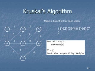
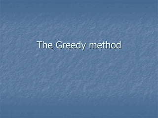
//v=set of vertices
//c=cost adjacency matrix of digraph G(V,E)
//n=number of vertices in given graph
//D[i]=contains current shortest path to vertex I
//c[i][j] is the cost of going from vertex I to j.If there is no path, assume
//c[i][j]= ∞ and c[i][j]=0
Algorithm Dijikstra(V,C,D,n)
{
s={1}
for i=2 to n do
d[i]=C[1,i]
for i=1 to n do
{
choose a vertex W in V-S such that D[W] is minimum
S=S U W //add W to S
for each vertex V in V-S d
D[V]=min(D[v],D[W],C[W[V])
}
}

Single-Source Shortest Path Problem
Single-Source Shortest Path Problem - The
problem of finding shortest paths from a source
vertex v to all other vertices in the graph.

Applications
- Maps (Map Quest, Google Maps)
- Routing Systems

Dijkstra's algorithm
Dijkstra's algorithm - is a solution to the single-source
shortest path problem in graph theory.
Works on both directed and undirected graphs. However,
all edges must have nonnegative weights.
Input: Weighted graph G={E,V} and source vertex v∈V,
such that all edge weights are nonnegative
Output: Lengths of shortest paths (or the shortest paths
themselves) from a given source vertex v∈V to all other
vertices

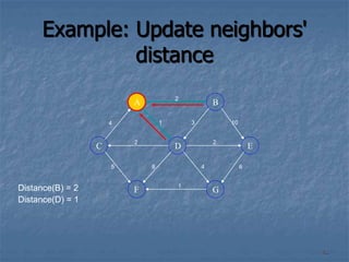
Approach
 The algorithm computes for each vertex v the distance
to v from the start vertex S, that is, the weight of a
shortest path between S and v.
 The algorithm keeps track of the set of vertices for
which the distance has been computed, called w
 Every vertex has a label D associated with it. For any
vertex v, D[v] stores an approximation of the distance
between v and w. The algorithm will update a D[v] value
when it finds a shorter path from w to v.
 When a vertex w is added to S, its label D[v] is equal to
the actual (final) distance between the starting vertex S
and vertex v.
39

40
Example: Initialization
A
G
F
B
E
C D
4 1
2
10
3
6
4
2
2
8
5
1
0
Pick vertex in List with minimum distance.
Distance(source) =0
S={A}
Find the nearest
vertex to source say w
i.e)D
V={A,B,C,D.E,F,G}

41
Example: Update neighbors'
distance
A
G
F
B
E
C D
4 1
2
10
3
6
4
2
2
8
5
1
Distance(B) = 2
Distance(D) = 1

42
Example: consider vertex with
minimum distance
Pick vertex in List with minimum distance, i.e., D
A
G
F
B
E
C D
4 1
2
10
3
6
4
2
2
8
5
1
0
1

43
Example: Update neighbors
A
G
F
B
E
C D
4 1
2
10
3
6
4
2
2
8
5
1
0 2
3 3
1
9 5
Distance(C) = 1 + 2 = 3
Distance(E) = 1 + 2 = 3
Distance(F) = 1 + 8 = 9
Distance(G) = 1 + 4 = 5
Use D as intermediate

44
Example: Continued...
A
G
F
B
E
C D
4 1
2
10
3
6
4
2
2
8
5
1
0 2
3 3
1
Pick vertex in List with minimum distance (B) and update neighbors
9 5
Note : distance(D) not
updated since D is
already known and
distance(E) not updated
since it is larger than
previously computed

45
A
G
F
B
E
C D
4 1
2
10
3
6
4
2
2
8
5
1
0 2
3 3
1
9 5
No updating
Pick vertex List with minimum distance (E) and update neighbors

46
A
G
F
B
E
C D
4 1
2
10
3
6
4
2
2
8
5
1
0 2
3 3
1
8 5
Pick vertex List with minimum distance (C) and update neighbors
Distance(F) = 3 + 5 = 8

47
A
G
F
B
E
C D
4 1
2
10
3
6
4
2
2
8
5
1
0 2
3 3
1
6 5
Distance(F) = min (8, 5+1) = 6
Previous distance
Pick vertex List with minimum distance (G) and update neighbors

48
Example (end)
A
G
F
B
E
C D
4 1
2
10
3
6
4
2
2
8
5
1
0 2
3 3
1
Pick vertex not in S with lowest cost (F) and update neighbors
6 5

Job sequencing with Deadline
 Job J1 J2 J3 J4 J5
 Deadline 2 1 3 2 1
 Profit 60 100 20 40 20
 Solution
 To solve this problem, the given jobs are sorted
according to their profit in a descending order.
Hence, after sorting, the jobs are ordered as
shown in the following table.

 Job J2 J1 J4 J3 J5
 Deadline 1 2 2 3 1
 Profit 100 60 40 20 20
 From this set of jobs, first we select J2, as it can be completed
within its deadline and contributes maximum profit.
 Next, J1 is selected as it gives more profit compared to J4.
 In the next clock, J4 cannot be selected as its deadline is over,
hence J3 is selected as it executes within its deadline.
 The job J5 is discarded as it cannot be executed within its deadline.
 Thus, the solution is the sequence of jobs (J2, J1, J3), which are
being executed within their deadline and gives maximum profit.

Unit 3-Greedy Method

Recommended

Recommended

More Related Content

What's hot

What's hot (20)

Similar to Unit 3-Greedy Method

Similar to Unit 3-Greedy Method (20)

More from DevaKumari Vijay

More from DevaKumari Vijay (20)

Recently uploaded

Recently uploaded (20)

Unit 3-Greedy Method