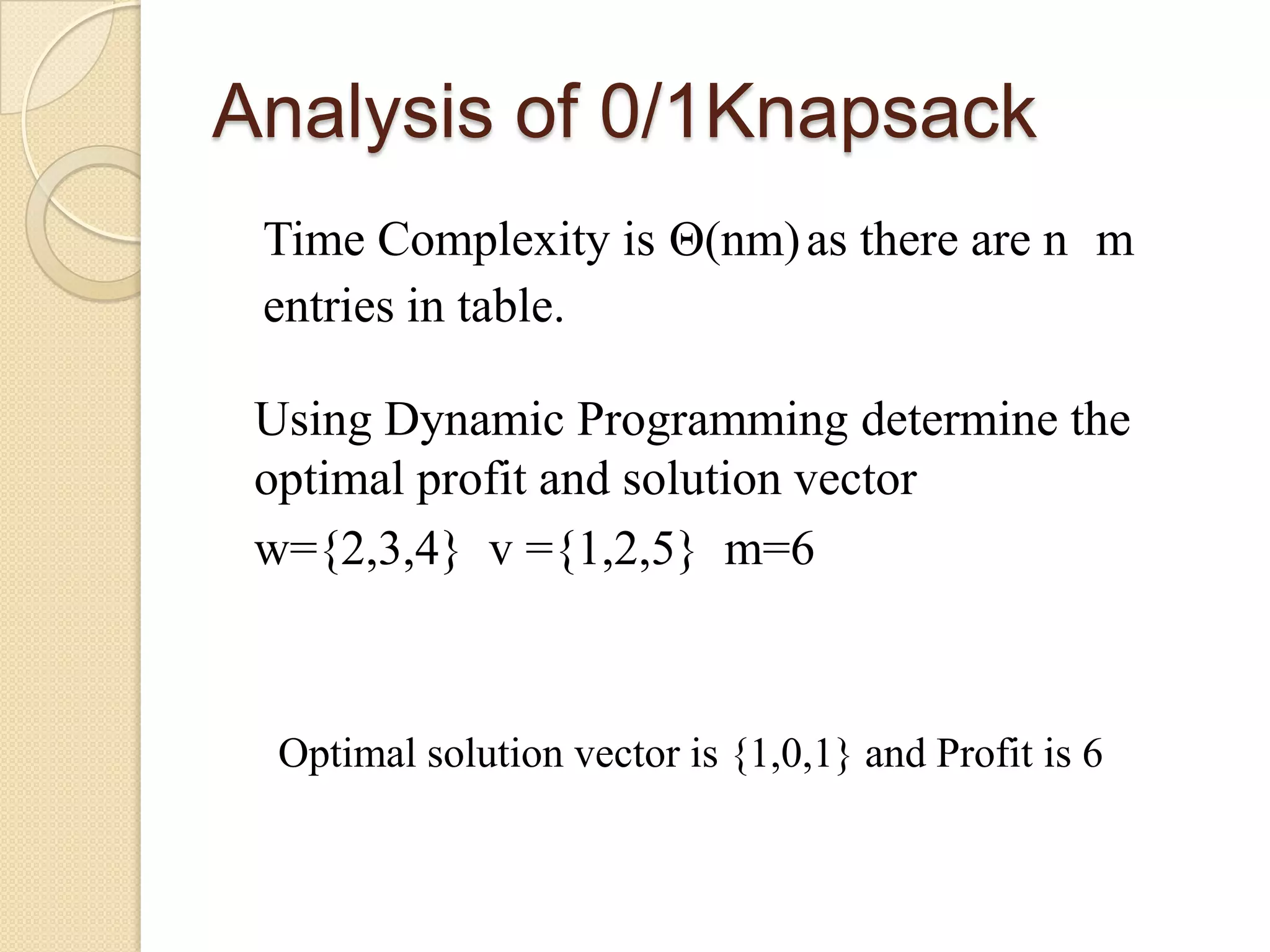
Dynamic programming is used to solve optimization problems by breaking them down into subproblems. It solves each subproblem only once, storing the results in a table to lookup when the subproblem recurs. This avoids recomputing solutions and reduces computation. The key is determining the optimal substructure of problems. It involves characterizing optimal solutions recursively, computing values in a bottom-up table, and tracing back the optimal solution. An example is the 0/1 knapsack problem to maximize profit fitting items in a knapsack of limited capacity.

1. Dynamic Programming

2. General Strategy
 Used for optimization problems: often minimizing or maximizing.
 Solves problems by combining solutions to sub-problems.
 Sub-problems are not independent.
 Reduces computation by
◦ Solving sub-problems in a bottom-up fashion.
◦ Storing solution to a sub-problem the first time it is solved.
◦ Looking up the solution when subproblem is encountered again.
 Key: determine structure of optimal solutions

3. Steps in Dynamic Programming
 Characterize structure of an optimal solution.
 Define value of optimal solution recursively.
 Compute optimal solution values caching in bottom-
up manner from table.
 Construct an optimal solution from computed values.

4. Principle of optimality
 Principle of optimality states that “ In an
optimal sequence of decisions or choices each
sub-sequences must be optimal.”
e.g. D
A
C B

5.  Suppose that in solving a problem, we have to make
a sequence of decisions D1, D2,…, Dn. Then
according to Principle of Optimality, if this
sequence is optimal, then the last k decisions,
1< k< n must be optimal.

6. Knapsack Problem
 A thief robbing a store and can carry a maximal weight of W into
their knapsack. There are n items and ith item weight wi and is
worth vi dollars. What items should thief take?
 Fractional Knapsack
◦ The items are allowed to be broken into smaller pieces so that
knapsack contains fraction of xi of item i, where 0 ≤ xi ≤ 1
 0/1 Knapsack
◦ Either to include an item in knapsack or to leave it (binary
choice), but may not take a fraction of an item i.e. 0 or 1.

7. 0/1 Knapsack Problem
Let i=1,2,3,…,n are items available.
wi - weight of ith item
vi – value of ith item
m – capacity of knapsack
 Now the problem is to maximize the value or profit with
capacity constraints
Let {x1,x2,…,xn} is the optimal solution
Where xi ∈ {0,1}

8. =0 if i=0 or j=0
=-∞ if j<0
C[i,j] =c[i-1,j] if wi ≥ 0
=max{vi+c[i-1,j-wi],c[i-1,wi]} if i>0 & j>wi
Consider the E.g. : w={1,2,5,6,7}
v={1,6,18,22,28}
m=11
How to calculate the cost table
C[1,1]=max{C[1-1,1-1]+1,C[1-1,1]}
=max{1,0}=1
C[1,2]=max{C[1-1,2-1]+1,C[1-1,1]}
=max{1,0}=1
C[3,3]=max{C[3-1,3-5]+18,C[3-1,3]}
=max{-∞,C[2,3]}
=C[2,3]

9.  Thus Optimal Solution Vector is, {0,0,1,1,0}
 And Optimal Profit is, 0+18+22+0=40

10. Dknap(i,j,m)
{
w :=[w1,w2,…,wn] ; // array of weights
v := [v1,v2,…,vn]; // array of values
C:= [1,2,…,n,1,2,…,m]; // Knapsack array(2-D)
// 1,2,…i,…,n are objects
// 1,2,…,j,…,m are capacities of knapsack

11. for i :=1 to n do
C[i,0]:=0; //Knapsack with capacity 0
for i:=1 to n do
{
for j:=1 to m do
{
if (i=1 and j<w[i]) then
C[i,j]=0;
else
if (i=1) then
C[i,j]=v[i];
else
if(j<w[i]) then
C[i,j]=C[i-1,j];
else
if(C[i-1,j] > C[i-1,j-w[i]]+v[i]) then
C[i,j]= C[i-1,j];
else
C[i,j]= C[i-1,j-w[i]]+v[i];
}
}
Traceback(C)
}

12. Traceback(C)
{ //opt[] array is used to store optimal solution vector
i:=n; j:=m;
while(i≥1)
{ k:=i; //k is the index of opt[] array
while(j≥0)
{
if(C[i,j]=C[i-1,j]) then
{
i:=i-1;
opt[k]:=0;
else
{
opt[k]=1;
i:=i-1;
j:=j-w[i];
}
}

13. Analysis of 0/1Knapsack
Time Complexity is Θ(nm) as there are n m
entries in table.
Using Dynamic Programming determine the
optimal profit and solution vector
w={2,3,4} v ={1,2,5} m=6
Optimal solution vector is {1,0,1} and Profit is 6