The document discusses various greedy algorithms including knapsack problems, minimum spanning trees, shortest path algorithms, and job sequencing. It provides descriptions of greedy algorithms, examples to illustrate how they work, and pseudocode for algorithms like fractional knapsack, Prim's, Kruskal's, Dijkstra's, and job sequencing. Key aspects covered include choosing the best option at each step and building up an optimal solution incrementally using greedy choices.

1. Greedy Method
Unit 3
Ms.Mary Jacob
Assistant Professor , Kristu Jayanti College , Bangalore

2.  In Greedy Method the problems have N inputs require us to obtain a subset
that satisfies few constraints.
 The greedy method is a simple strategy of progressively building up a
solution, one element at a time, by choosing the best possible element at
each stage.
 At each stage, a decision is made regarding whether or not a particular input
is in an optimal solution.
 The Greedy method is used for solving optimization problems. Every
greedy method based problem will be given a set of inputs and constraints.
The objective is to find a solution vector, which satisfies the constraint.
Greedy Method

3.  Some of the important concepts of greedy method are:
 Feasible solution: Any subset of the original input that satisfies a given set
of constraints is called a feasible solution.
 Optimal solution: An optimal solution is one, which maximizes or
minimizes the given objective function.
Greedy Method

4.  In Greedy Method the problems have N inputs require us to obtain a subset
that satisfies few constraints.
 The greedy method is a simple strategy of progressively building up a solution,
one element at a time, by choosing the best possible element at each stage.
 At each stage, a decision is made regarding whether or not a particular input is
in an optimal solution.
 This is done by considering the inputs in an order determined by some
selection procedure. If the inclusion of the next input, into the partially
constructed optimal solution will result in an infeasible solution then this input
is not added to the partial solution. The selection procedure is based on some
optimization measure.
 Most of them, however, will result in algorithms that generate sub-optimal
solutions. This version of greedy technique is called subset paradigm.
Greedy Method - Subset Paradigm

5.  For the problems that make decisions by considering the inputs in some
order, each decision is made using an optimization criterion that can be
computed using decisions already made. This version of greedy method is
ordering paradigm.
 Some problems like optimal storage on tapes, optimal merge patterns and
single source shortest path are based on ordering paradigm.
Greedy Method-Ordering Paradigm

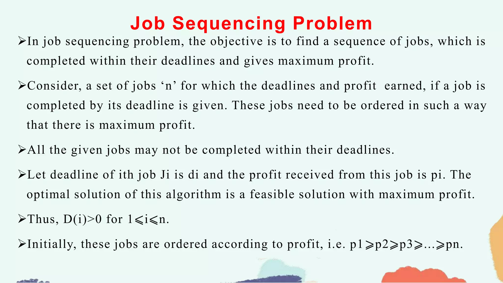
6. Control Abstraction of Greedy method
Control Abstraction of Greedy method
Algorithm Greedy(a,n)
{
a[n] //array a with n inputs
solution := 0 //initialize the solution
for i:=1 to n do
{
x = select (a)
if Feasible (solution, x) then
solution:=union(solution, x);
}
return solution;
}

7. Knapsack Problem
 This problem is commonly known as the knapsack or the rucksack problem.
 There are different kinds of items and each item has a weight and profit value
associated with it.
 The problem is to pick up items with the limitation of maximum weight the
knapsack can hold and maximizing the profit.

8. Knapsack Problem - Variations
 0-1Knapsack Problem → When we are not available to just pick a part of an item
i.e., we either take the entire item or not and can't just break the item and take some
fraction of it, then it is called integer knapsack problem.
 Fractional Knapsack Problem → Here, we can take even a fraction of any item.
 Bounded Knapsack Problem (BKP) → In this case, the quantity of each item can
exceed 1 but can't be infinitely present i.e., there is an upper bound on it.
So, 0≤xi≤c0≤xi≤c, where c is the maximum quantity of xi we can take.
 Unbounded Knapsack Problem (UKP) → Here, there is no limitation on the
quantity of a specific item we can take i.e., xi≥0

9. Knapsack Problem
We are given a knapsack (bag or a container) of capacity m and n objects of weight w1,
w2…..wn with profit p1, p2 ,….pn.
Objective: Fill the knapsack which maximises the profit earned and the output is a
vector xi where 1 <= i <= n. It is a maximization problem.
Constraints: The total capacity cannot exceed m at any point of time.
The problem can be stated as,
Max ∑ pi xi
1<= i <=n
Subject to ∑ wi xi <= m
1<= i <=n

10. Knapsack Fraction-Problem

11. Knapsack Fraction-Problem

12. Knapsack Fraction-Problem

13. Knapsack Fraction-Problem
The Feasible solutions are 31, 28, 31.5, 28
The Optimal solution is 31.5

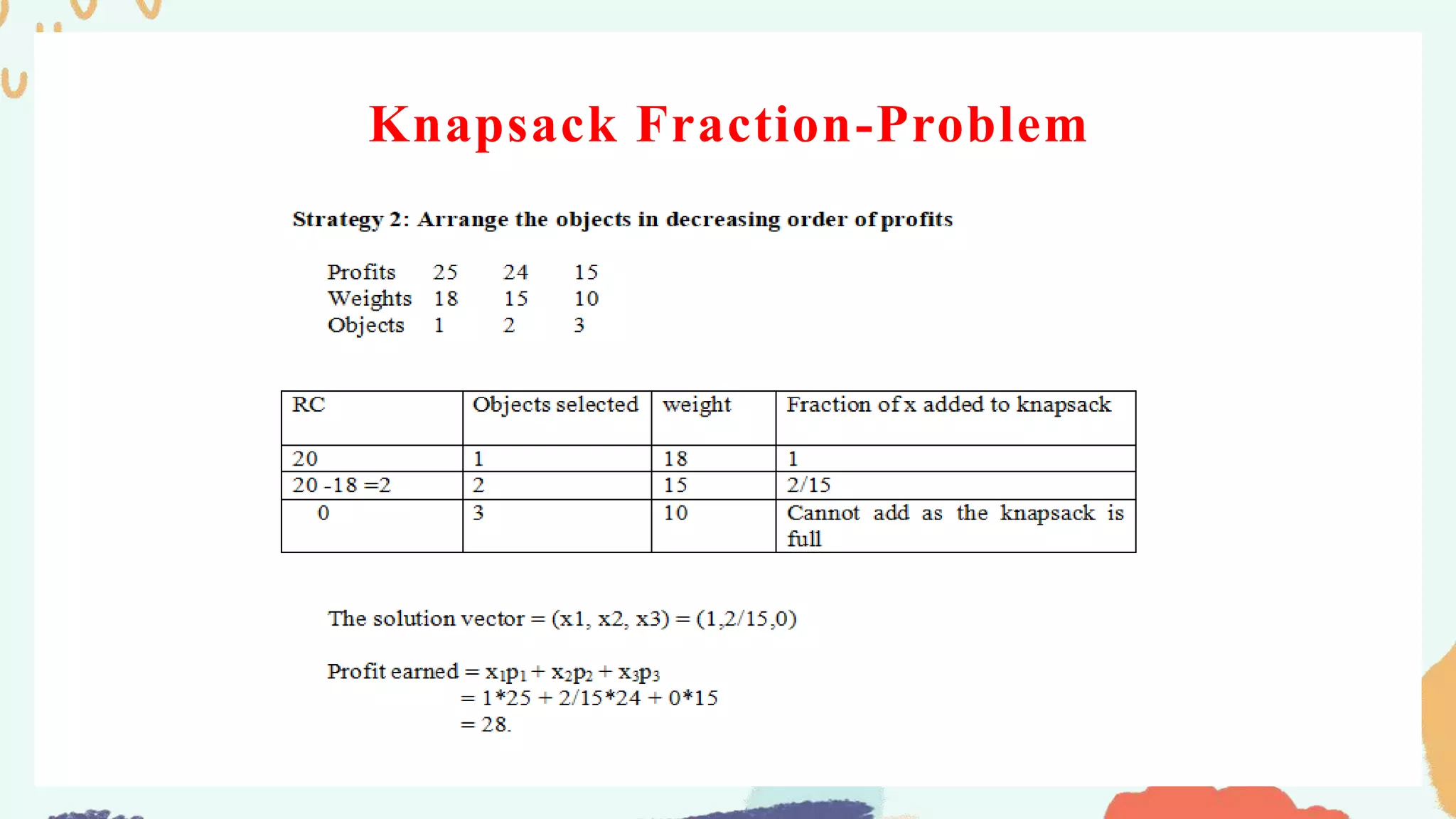
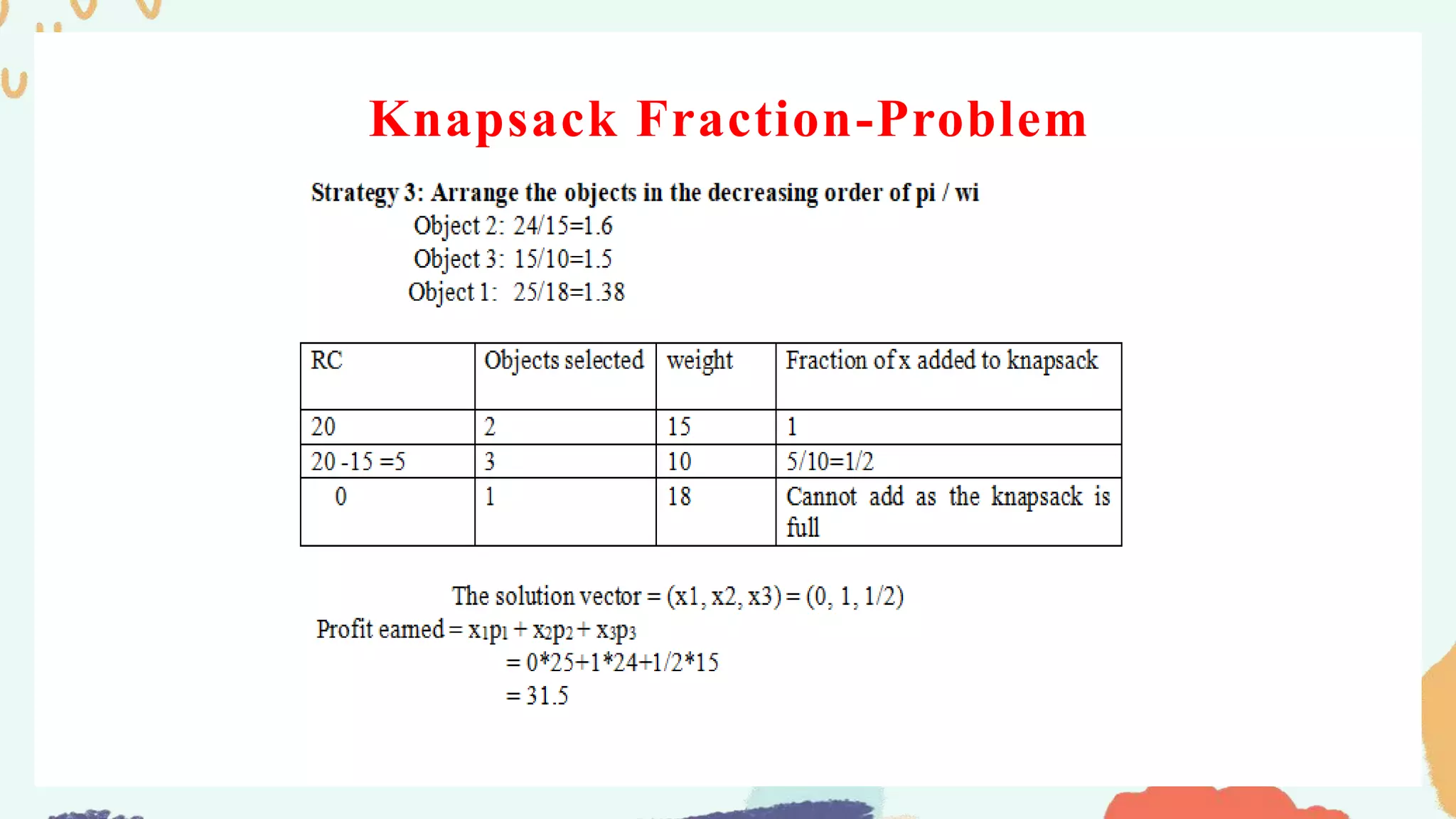
14. Knapsack Fraction-Algorithm
Algorithm: Greedyknapsack fraction(M, n, w, P, x)
Assume the objects to be arranged in decreasing order of pi / wi. Let M be the knapsack capacity, n is the
number of edges, w [1 : n] is the array of weights, P[1 : n]is the array of profits ,x is a solution vector.
Step 1: Remaining capacity RC =m
Step 2: Repeat for i=1 to n do
x[i] = 0
end for
Step 3: Repeat for i==1 to n do
if (w[ i ] < RC)
x[ i ]=1
RC=RC-w[ i ]
Step 4: else
x[ i ]=RC/w[ i ]
break
End for
Step 5: For i=1 to n do
sum=sum+p [ i ]*x[ i ]
End for

15. Knapsack 0/1-Algorithm
Algorithm: Greedyknapsack0/1(M, n, w, P, x)
Assume the objects to be arranged in decreasing order of pi / wi. Let M be the knapsack capacity, n is the
number of edges, w [1 : n] is the array of weights, P[1 : n]is the array of profits ,x is a solution vector.
Step 1: Remaining capacity RC =m
Step 2: Repeat for i=1 to n do
x[i] = 0
end for
Step 3: Repeat for i=1 to n do
if (w[ i ] < RC)
x[ i ]=1
RC=RC- w[ i ]
Step 4: else
x[ i ]= 0
break
End for
Step 5: For i=1 to n do
sum=sum+p [ i ]*x[ i ]
End for

16. Knapsack Problem - 0/1 Approach
Example :
For the knapsack problem n=4,m=40 (p1,p2,p3,p4) = (20,40, 35,45) and
(w1,w2,w3,w4) = (20,25,10,15).Find the feasible solutions and optimal solution using
greedy method.

17. Minimum cost Spanning tree(MST)
A spanning tree for a connected undirected graph G=(V, E) is a sub graph
of G that is undirected tree and contains all the vertices of G.
A spanning tree should contain all the vertices and a subset of edges. In a
weighted graph G=(V,E) the weight W of a sub graph is the sum of the
edges in the sub graph.
 A minimum spanning tree for a weighted graph is spanning tree with
minimum weight.
No cycles in Spanning tree

18. Minimum cost Spanning tree(MST)
The two popular algorithms to find the minimum cost spanning tree are,
 Kruskal’s Algorithm
 Prim’s Algorithm

19. Prim’s algorithm
Prim’s Algorithm is used to find the minimum spanning tree of a given
graph through a sequence of expanding sub trees.
The initial sub tree is a sequence consisting of some arbitrary vertex
selected from the set V , of graph vertices.
On each iteration the current tree is expanded by simply attaching it to
the nearest vertex (minimum cost edge vertex).
The algorithm stops after all the vertices have been included in the
spanning tree being constructed.

20. Prim’s algorithm
Algorithm :Prim’s(n, c)
//Assume G is connected, undirected and weighted graph.
//Input : The cost adjacency matrix C and number of vertices n.
//Output: Minimum weight spanning tree.
for i=1 to n do
visited [ i ]=0
u=1
visited [ u ] = 1
while( there is still an unchosen vertex ) do
Let <u, v> be the lightest edge between any chosen vertex u and unchosen vertex v
visited [ v ] =1
T=union (T, <u,v>)
end while
return T

21. Kruskal’s Algorithm
Let G= (V, E) be a directed graph . This algorithm selects n-1 edges one at
time. The algorithm selects the least cost edge (u, v) from E and deletes the
edge (u, v) from E.
Then it checks whether the selected edge (u,v) results in a cycle when added to
the list of already selected edges to form a MST.
 If no cycles are formed, the selected edge is added to the list of edges selected
to form a MST.
The selected edge which results in a cycle are neglected .The procedure is
repeated till all n-1 edges are selected and there are no more edges to consider

22. Kruskal’s Algorithm
Algorithm : Kruskal’s (E,n)
//Let E be the list of edges
//n be the number of vertices in the given graph.
Sort E in the increasing order of their edge weights
Initially T = 0
while ( T doesnot contain n – 1 edges)
find the minimum cost edge not yet considered in E and call it as <u, v>
if( <u, v> does not form a cycle
T= T + <u, v>
else
delete <u , v>
end while
return (T)

23. Dijikstra’s Single Source Shortest Path Algorithm
Dijikstra’s Single-source shortest path algorithm finds the shortest path from
the the single source to all other nodes.
Algorithm
1) Create a set S (shortest path tree set) that keeps track of vertices
included in shortest path tree, i.e., whose minimum distance from source is
calculated and finalized. Initially, this set is empty.
2) Assign a distance value to all vertices in the input graph.
3) While S doesn’t include all vertices
….a) Pick a vertex w which is not there in S and has minimum distance
value.
….b) Include w to S.
….c) Update distance value of all adjacent vertices of w. To update the
distance values, iterate through all adjacent vertices. For every adjacent
vertex w, if sum of distance value of s (from source) and weight of edge w-v,
is less than the distance value of v, then update the distance value of v.

24. Algorithm-Dijikstra’s Single Source Shortest Path
dist[S] ← 0 // The distance to source vertex is set to 0
Π[S] ← NIL // The predecessor of source vertex is set as NIL
for all v ∈ V - {S} // For all other vertices
do dist[v] ← ∞ // All other distances are set to ∞
Π[v] ← NIL // The predecessor of all other vertices is set as NIL
S ← ∅ // The set of vertices that have been visited 'S' is
initially empty
Q ← V // The queue 'Q' initially contains all the vertices
while Q ≠ ∅ // While loop executes till the queue is not empty
do u ← mindistance (Q, dist) // A vertex from Q with the least distance is selected
S ← S ∪ {u} // Vertex 'u' is added to 'S' list of vertices that have
been visited
for all v ∈ neighbors[u] // For all the neighboring vertices of vertex 'u'
do if dist[v] > dist[u] + w(u,v) // if any new shortest path is discovered
then dist[v] ← dist[u] + w(u,v) // The new value of the shortest path is selected
return dist

25. Job Sequencing Problem
In job sequencing problem, the objective is to find a sequence of jobs, which is
completed within their deadlines and gives maximum profit.
Consider, a set of jobs ‘n’ for which the deadlines and profit earned, if a job is
completed by its deadline is given. These jobs need to be ordered in such a way
that there is maximum profit.
All the given jobs may not be completed within their deadlines.
Let deadline of ith job Ji is di and the profit received from this job is pi. The
optimal solution of this algorithm is a feasible solution with maximum profit.
Thus, D(i)>0 for 1⩽i⩽n.
Initially, these jobs are ordered according to profit, i.e. p1⩾p2⩾p3⩾...⩾pn.

26. Job Sequencing Problem
Algorithm
Sort the jobs based on decreasing order of profit.
Iterate through the jobs and perform the following:
Choose a Slot i if:
Slot i isn’t previously selected.
I < deadline
I is maximum
If no such slot exists, ignore the job and continue.

27. Job Sequencing Problem
Example
Given 5 Jobs with deadline={2, 1, 3, 2, 1}
Profit= { 60, 100, 20, 40, 20 }
Job J1 J2 J3 J4 J5
Deadline 2 1 3 2 1
Profit 60 100 20 40 20

28. Solution
Job J2 J1 J4 J3 J5
Deadline 1 2 2 3 1
Profit 100 60 40 20 20
1. J2 is selected as it cab be completed within its deadline-1 and
contributes maximum profit.
2. J1 is selected next as it gives more profit compared to J4 and deadline -
2 can be achieved
3. J4 cannot be selected as its deadline=2 is over
4. J3 is selected as it executes within its deadline=3.
5. J5 is also not selected as it cannot be executed within its deadline=3
Optimal solution is the sequence of jobs (J2, J1, J3), which are being
executed within their deadline and gives maximum profit=
100 + 60 + 20 = 180

29. THANKS