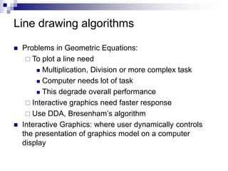
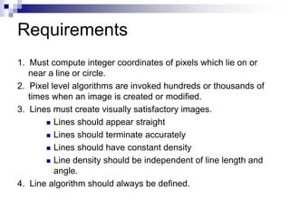
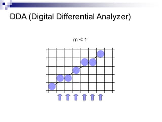
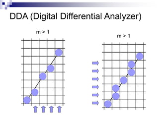
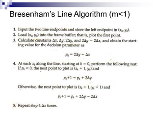
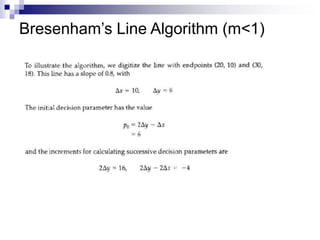
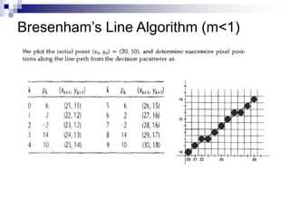
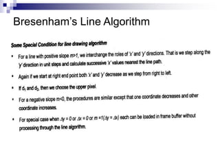
Scan Conversion
Dept of Computer Science & Engineering
Islamic University, Kushtia
Graphics Primitives
 The basic building blocks for pictures are referred to as output
primitives.
 They include:
 character strings and
 geometric entities,
 Points,
 Straight lines,
 Curved Lines,
 Circle, Ellipse
 Filled areas (polygons, circles, etc.), and
 Shapes defined with arrays of color points.
 Routines for generating output primitives provide the basic
tools for constructing pictures.
Coordinates
Pixel addressing in raster graphics
Pixel
address
Pixel
x x+1 x+2 x+3 x+4
y
y+1
y+2
y+3
Theoretical length
Actual length
POINTS AND LINES
 Point plotting is accomplished by converting a single
coordinate position furnished by an application program
into appropriate operations for the output device in use.
 For example, CRT monitor, the electron beam is
turned on to illuminate the screen phosphor at the
selected location
POINTS AND LINES
 Line drawing is accomplished by calculating
intermediate positions along the line path
between two specified endpoint positions.
 Digital devices display a straight line segment by
plotting discrete points between the two
endpoints.
Discrete coordinate positions along the line
path are calculated from the equation of the
line.
Theoretical Line
Line on Display Devices
Line drawing algorithms
 Geometric
 Display devices
 DDA
 Bresenham
Line drawing algorithms
 The Cartesian slope-intercept
equation for a straight line is
 with m representing the slope of
the line and b as they intercept
Line drawing algorithms
 Problems in Geometric Equations:
 To plot a line need
 Multiplication, Division or more complex task
 Computer needs lot of task
 This degrade overall performance
 Interactive graphics need faster response
 Use DDA, Bresenham’s algorithm
 Interactive Graphics: where user dynamically controls
the presentation of graphics model on a computer
display
Requirements
1. Must compute integer coordinates of pixels which lie on or
near a line or circle.
2. Pixel level algorithms are invoked hundreds or thousands of
times when an image is created or modified.
3. Lines must create visually satisfactory images.
 Lines should appear straight
 Lines should terminate accurately
 Lines should have constant density
 Line density should be independent of line length and
angle.
4. Line algorithm should always be defined.
DDA (Digital Differential Analyzer)
m < 1
DDA (Digital Differential Analyzer)
m > 1
m > 1
DDA Algorithms
 DDA is a scan-conversion line algorithm based on
calculating either y or x
 If the slope is less than or equal to 1, we sample at unit x
intervals ( x = 1) and compute each successive y value
as
where k=1 for first point and increases by 1until the final
endpoint is reached
 Calculated y values must be rounded to the nearest
integer
DDA Algorithms
 For lines with a positive slope greater than 1, reverse the
roles of x and y.
 we sample at unit y intervals (y = 1) and calculate
each succeeding x value as
equation (a) and (b) are based on the assumption that
lines are to be processed from the left endpoint to the
right endpoint
DDA Algorithms
 If this processing is reversed, that is from right to left
 The DDA algorithm is a faster method for calculating
pixel positions than the direct use
 It eliminates the multiplication by making use of raster
characteristics
DDA at a glance
 input line endpoints, (x1,y1) and (x2, y2)
 set pixel at position (x1,y1)
 calculate slope m
 Case |m|≤1: repeat the following steps until (x2, y2) is
reached:
yi+1 = yi + y/ x
xi+1 = xi + 1
set pixel at position (xi+1,Round(yi+1))
 Case |m|>1: repeat the following steps until (x2, y2) is
reached:
xi+1 = xi + x/ y
yi+1 = yi + 1
set pixel at position (Round(xi+1), yi+1)
Bresenham’s Line Algorithm
 Bresenham’s scan converts lines using only incremental
integer calculations that can be adapted to display
circles and other curves.
|m|<1 |m|>1
Bresenham’s Line Algorithm
|m|<1
Bresenham’s Line Algorithm (m<1)
 Starting from the left endpoint (x0, y0) of a given line,
 We step to each successive column (x position) and
 Plot the pixel whose scan-line y value is closest to the
line path.
 Let we have determined the pixel at (xk, yk) to be
displayed,
 we next need to decide which pixel to plot in column
xk+1,
 Our choices are the pixels at positions (xk+1, yk) and
(xk+1, yk+1)
Bresenham’s Line Algorithm
d1
d2
xk xk+1=x+1
yk
y = m(x+1) + b
y = mx + b
yk+1=y+1
Bresenham’s Line Algorithm
 They coordinate on the mathematical line at pixel column
position xk+1 is calculated as
 The difference between these two separations is
Bresenham’s Line Algorithm
where pk = x(d1 – d2) is decision parameter for the kth
step in the line algorithm
The sign of p, is the same as the sign of (d1 – d2) since
x > 0
and c is constant and c = 2y + x(2b – 1),
Bresenham’s Line Algorithm
 If (d1 < d2) then pk is negative
 We plot lower pixel (xk+1, yk)
 If (d1  d2) then pk is positive
 We plot lower pixel (xk+1, yk+1)
 For next decision parameter pk+1
 Increment x as xk+1 = xk+1
Bresenham’s Line Algorithm
 The term (yk+1–yk) of eq-(f) either 0 or 1 depending on
sign of pk
Bresenham’s Line Algorithm
 If pk < 0 true line close to lower pixel and yk +1 = yk
pk+1 = pk + 2y -- g(a)
 If pk  0 true line close to lower pixel and yk +1 = yk+1
pk+1 = pk + 2y – 2x -- g(b)
 First decision parameter p0 from eq-(d) as considering the line
start from (0, 0) as
p0 = 2y.0 – 2x.0 + c
p0 = c = 2y + x(2b – 1)
but y = mx + b or b = 0
p0 = 2y - x
Bresenham’s Line Algorithm (m<1)
Bresenham’s Line Algorithm

03.Scan Conversion.ppt

  • 1.
    Scan Conversion Dept ofComputer Science & Engineering Islamic University, Kushtia
  • 2.
    Graphics Primitives  Thebasic building blocks for pictures are referred to as output primitives.  They include:  character strings and  geometric entities,  Points,  Straight lines,  Curved Lines,  Circle, Ellipse  Filled areas (polygons, circles, etc.), and  Shapes defined with arrays of color points.  Routines for generating output primitives provide the basic tools for constructing pictures.
  • 3.
  • 4.
    Pixel addressing inraster graphics Pixel address Pixel x x+1 x+2 x+3 x+4 y y+1 y+2 y+3 Theoretical length Actual length
  • 5.
    POINTS AND LINES Point plotting is accomplished by converting a single coordinate position furnished by an application program into appropriate operations for the output device in use.  For example, CRT monitor, the electron beam is turned on to illuminate the screen phosphor at the selected location
  • 6.
    POINTS AND LINES Line drawing is accomplished by calculating intermediate positions along the line path between two specified endpoint positions.  Digital devices display a straight line segment by plotting discrete points between the two endpoints. Discrete coordinate positions along the line path are calculated from the equation of the line.
  • 7.
  • 8.
  • 9.
    Line drawing algorithms Geometric  Display devices  DDA  Bresenham
  • 10.
    Line drawing algorithms The Cartesian slope-intercept equation for a straight line is  with m representing the slope of the line and b as they intercept
  • 11.
    Line drawing algorithms Problems in Geometric Equations:  To plot a line need  Multiplication, Division or more complex task  Computer needs lot of task  This degrade overall performance  Interactive graphics need faster response  Use DDA, Bresenham’s algorithm  Interactive Graphics: where user dynamically controls the presentation of graphics model on a computer display
  • 12.
    Requirements 1. Must computeinteger coordinates of pixels which lie on or near a line or circle. 2. Pixel level algorithms are invoked hundreds or thousands of times when an image is created or modified. 3. Lines must create visually satisfactory images.  Lines should appear straight  Lines should terminate accurately  Lines should have constant density  Line density should be independent of line length and angle. 4. Line algorithm should always be defined.
  • 13.
  • 14.
    DDA (Digital DifferentialAnalyzer) m > 1 m > 1
  • 15.
    DDA Algorithms  DDAis a scan-conversion line algorithm based on calculating either y or x  If the slope is less than or equal to 1, we sample at unit x intervals ( x = 1) and compute each successive y value as where k=1 for first point and increases by 1until the final endpoint is reached  Calculated y values must be rounded to the nearest integer
  • 16.
    DDA Algorithms  Forlines with a positive slope greater than 1, reverse the roles of x and y.  we sample at unit y intervals (y = 1) and calculate each succeeding x value as equation (a) and (b) are based on the assumption that lines are to be processed from the left endpoint to the right endpoint
  • 17.
    DDA Algorithms  Ifthis processing is reversed, that is from right to left  The DDA algorithm is a faster method for calculating pixel positions than the direct use  It eliminates the multiplication by making use of raster characteristics
  • 18.
    DDA at aglance  input line endpoints, (x1,y1) and (x2, y2)  set pixel at position (x1,y1)  calculate slope m  Case |m|≤1: repeat the following steps until (x2, y2) is reached: yi+1 = yi + y/ x xi+1 = xi + 1 set pixel at position (xi+1,Round(yi+1))  Case |m|>1: repeat the following steps until (x2, y2) is reached: xi+1 = xi + x/ y yi+1 = yi + 1 set pixel at position (Round(xi+1), yi+1)
  • 19.
    Bresenham’s Line Algorithm Bresenham’s scan converts lines using only incremental integer calculations that can be adapted to display circles and other curves. |m|<1 |m|>1
  • 20.
  • 21.
    Bresenham’s Line Algorithm(m<1)  Starting from the left endpoint (x0, y0) of a given line,  We step to each successive column (x position) and  Plot the pixel whose scan-line y value is closest to the line path.  Let we have determined the pixel at (xk, yk) to be displayed,  we next need to decide which pixel to plot in column xk+1,  Our choices are the pixels at positions (xk+1, yk) and (xk+1, yk+1)
  • 22.
    Bresenham’s Line Algorithm d1 d2 xkxk+1=x+1 yk y = m(x+1) + b y = mx + b yk+1=y+1
  • 23.
  • 24.
    Bresenham’s Line Algorithm They coordinate on the mathematical line at pixel column position xk+1 is calculated as  The difference between these two separations is
  • 25.
    Bresenham’s Line Algorithm wherepk = x(d1 – d2) is decision parameter for the kth step in the line algorithm The sign of p, is the same as the sign of (d1 – d2) since x > 0 and c is constant and c = 2y + x(2b – 1),
  • 26.
    Bresenham’s Line Algorithm If (d1 < d2) then pk is negative  We plot lower pixel (xk+1, yk)  If (d1  d2) then pk is positive  We plot lower pixel (xk+1, yk+1)  For next decision parameter pk+1  Increment x as xk+1 = xk+1
  • 27.
    Bresenham’s Line Algorithm The term (yk+1–yk) of eq-(f) either 0 or 1 depending on sign of pk
  • 28.
    Bresenham’s Line Algorithm If pk < 0 true line close to lower pixel and yk +1 = yk pk+1 = pk + 2y -- g(a)  If pk  0 true line close to lower pixel and yk +1 = yk+1 pk+1 = pk + 2y – 2x -- g(b)  First decision parameter p0 from eq-(d) as considering the line start from (0, 0) as p0 = 2y.0 – 2x.0 + c p0 = c = 2y + x(2b – 1) but y = mx + b or b = 0 p0 = 2y - x
  • 29.
  • 30.
  • 31.
  • 32.