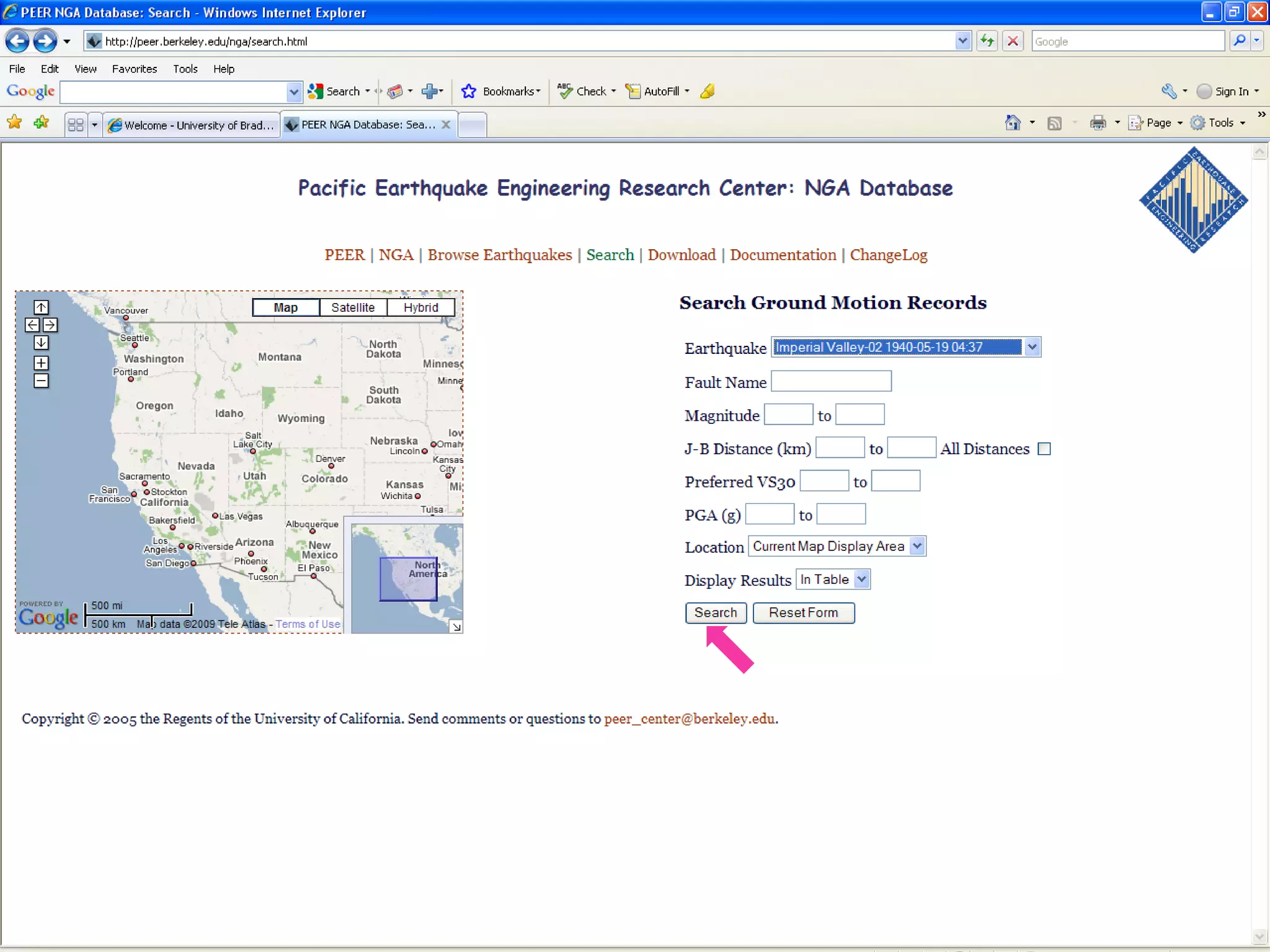
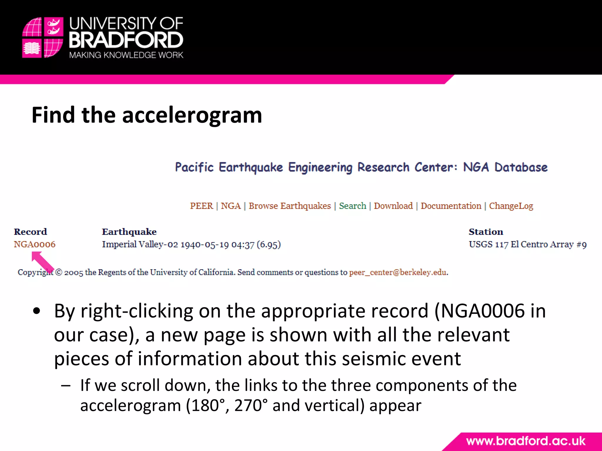
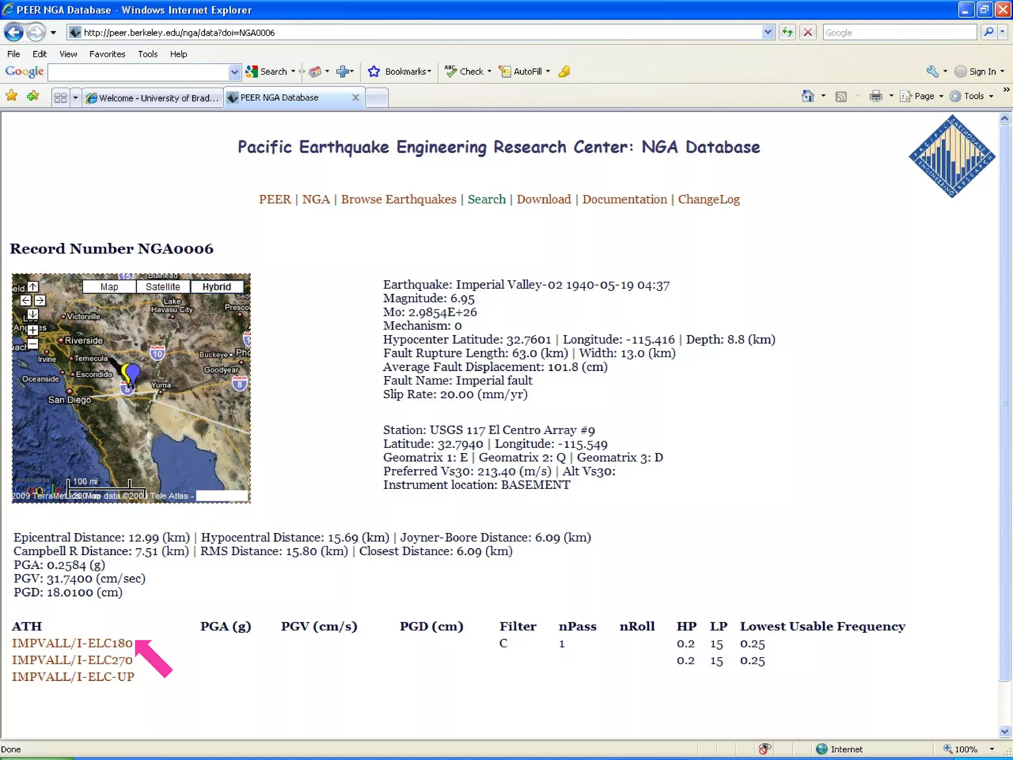
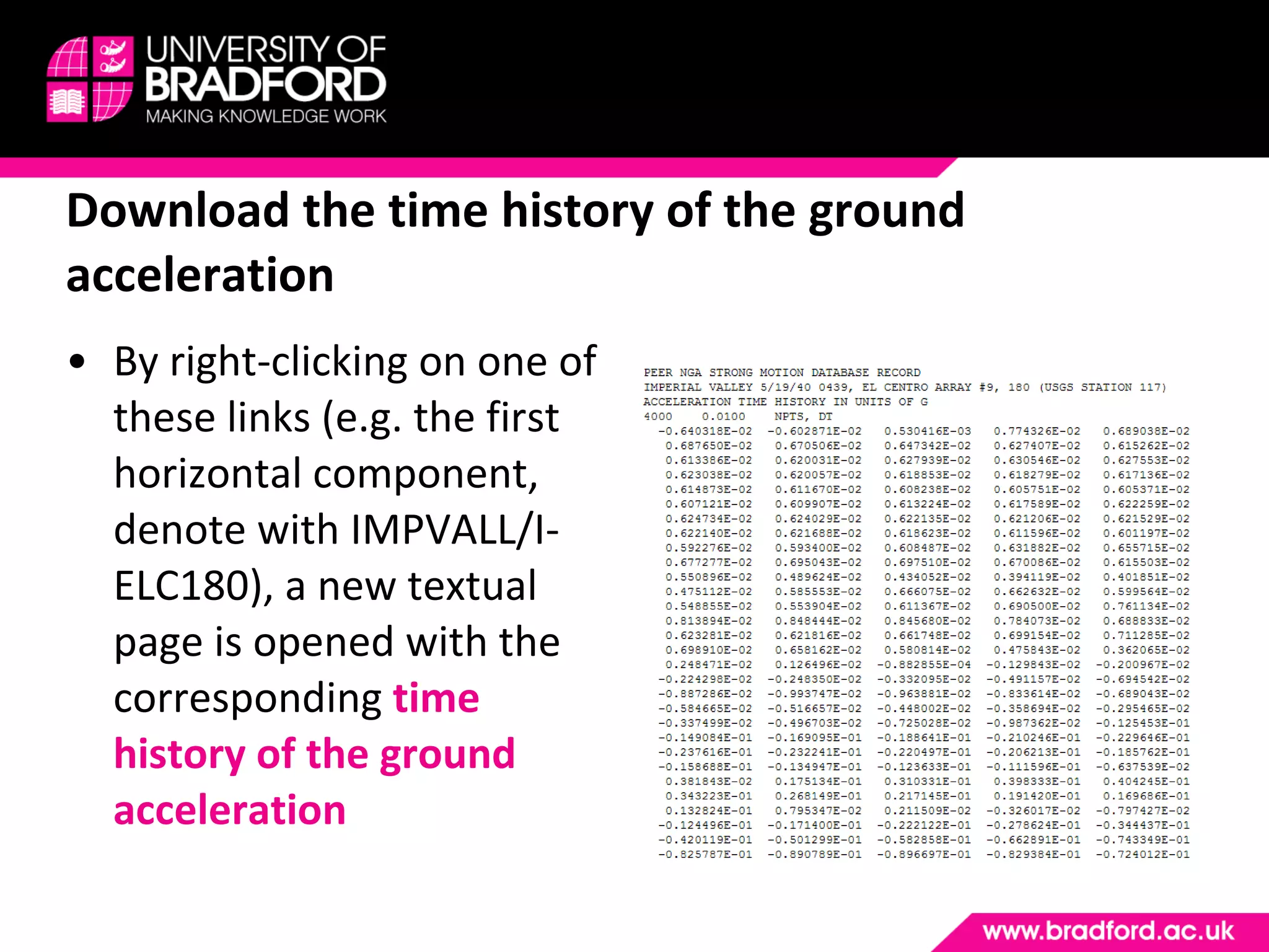
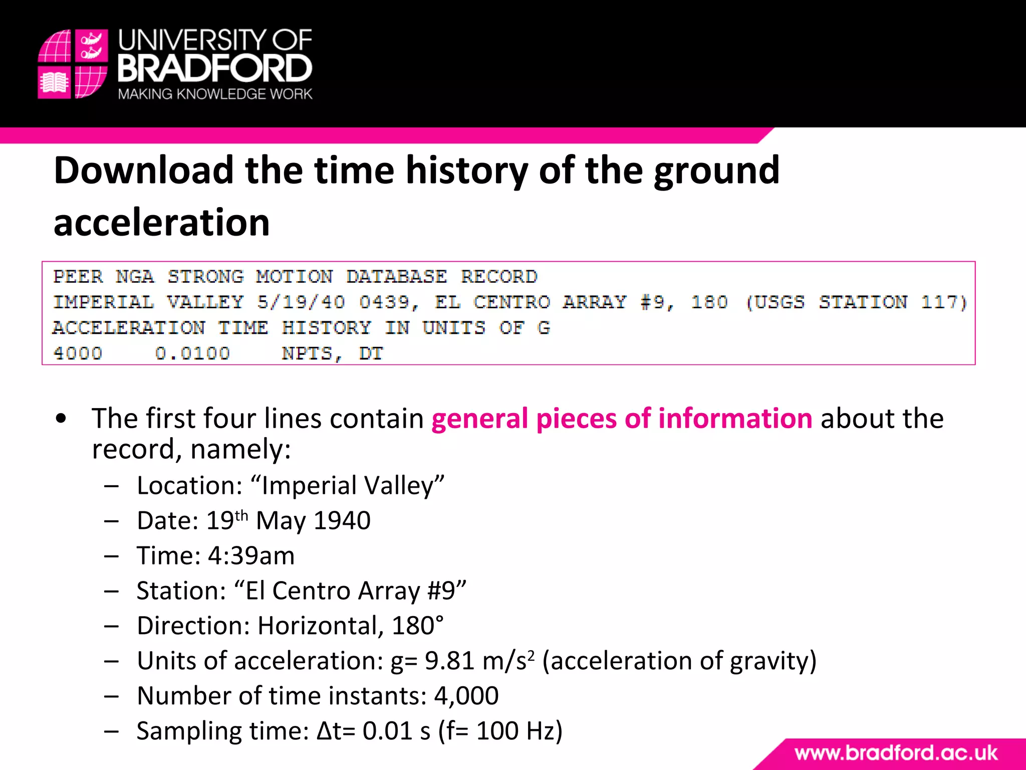
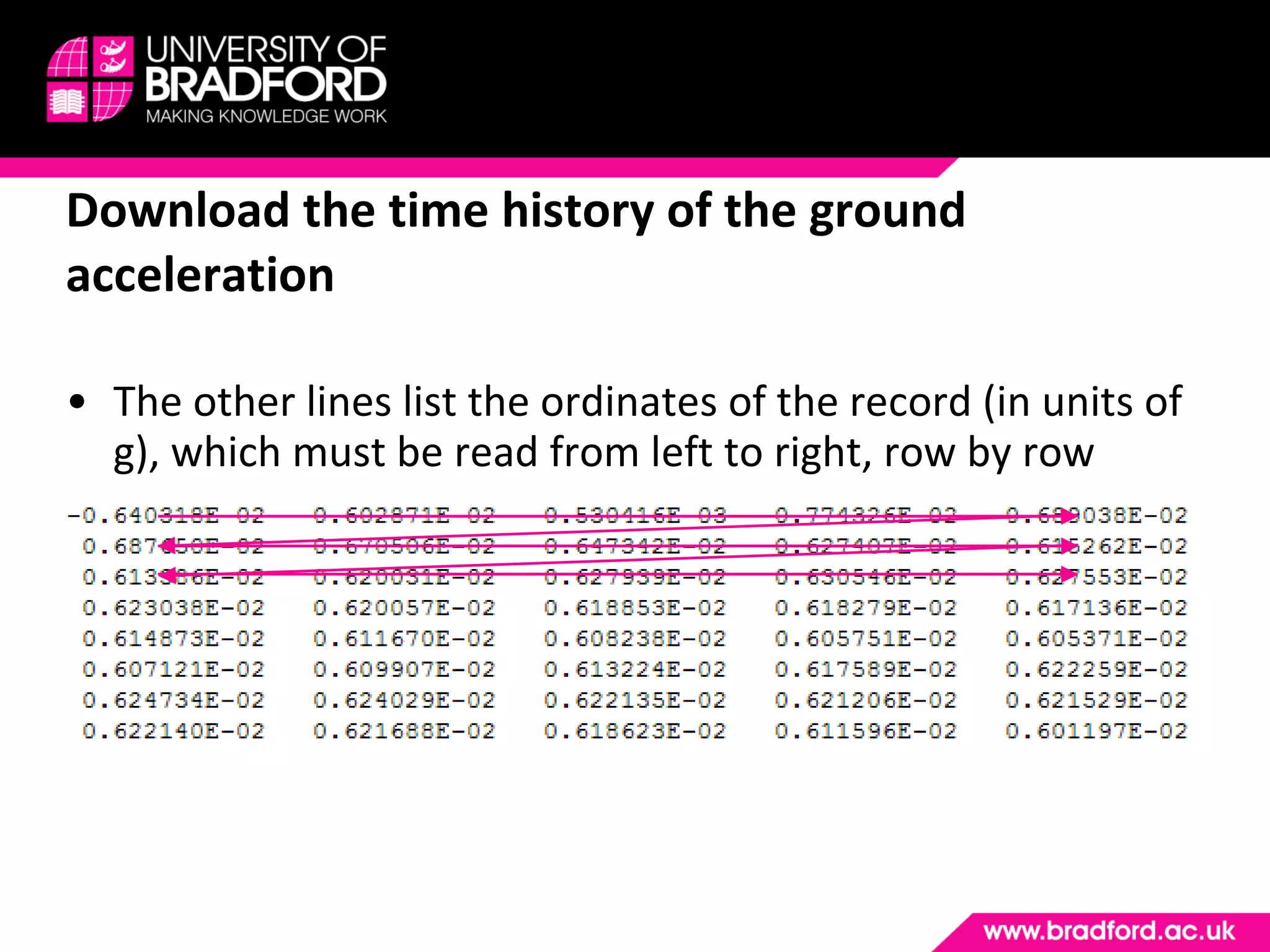
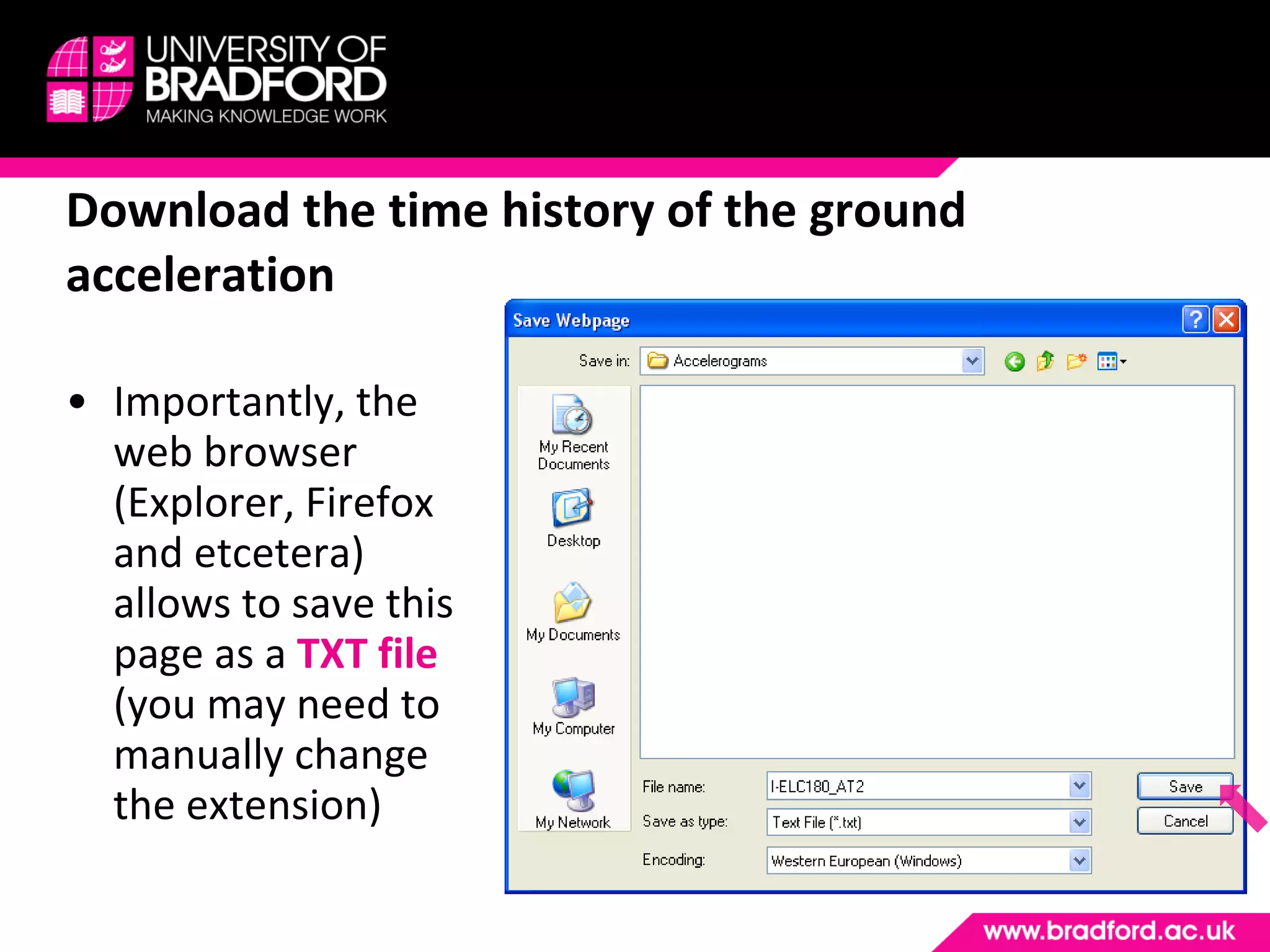
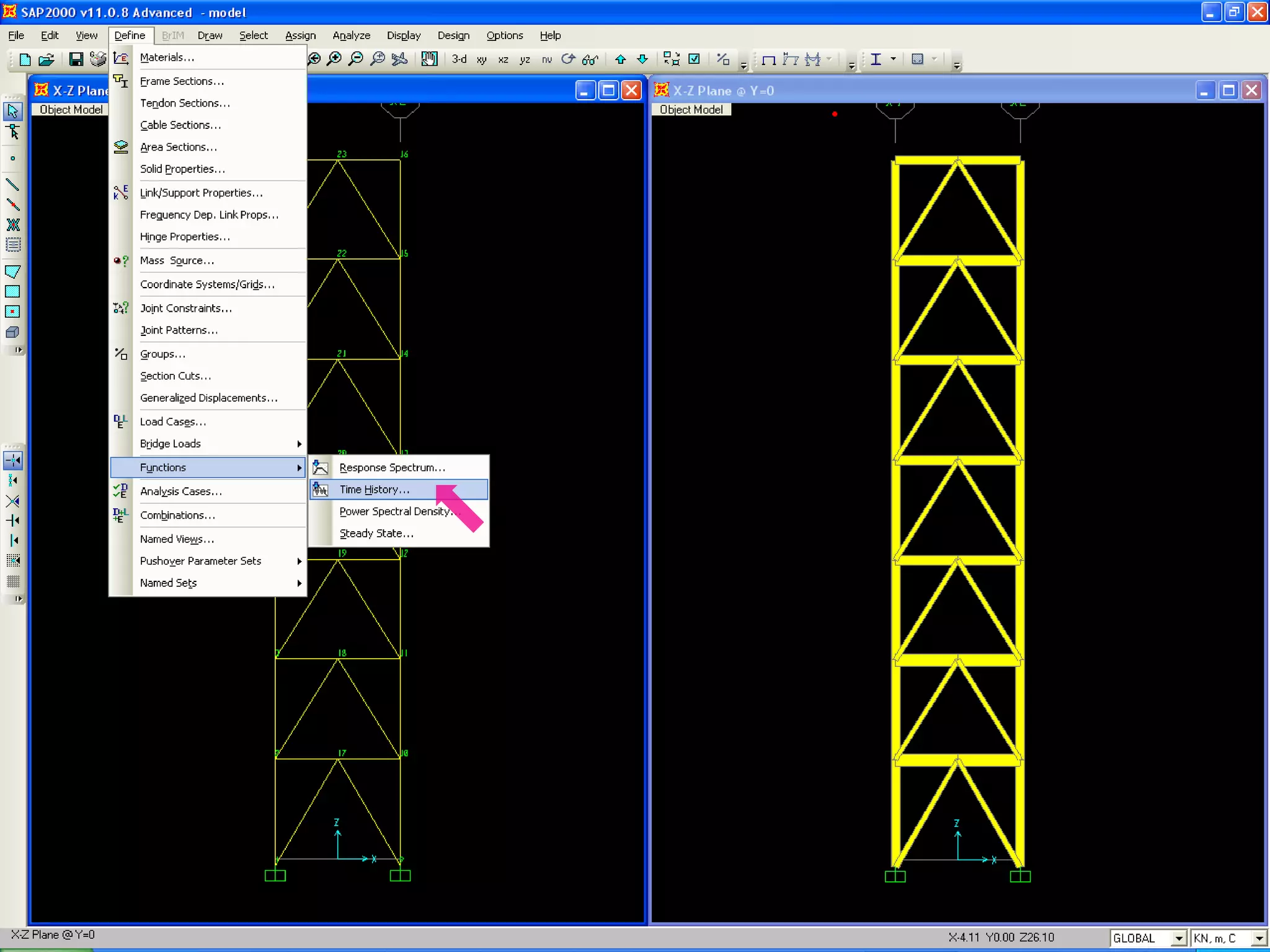
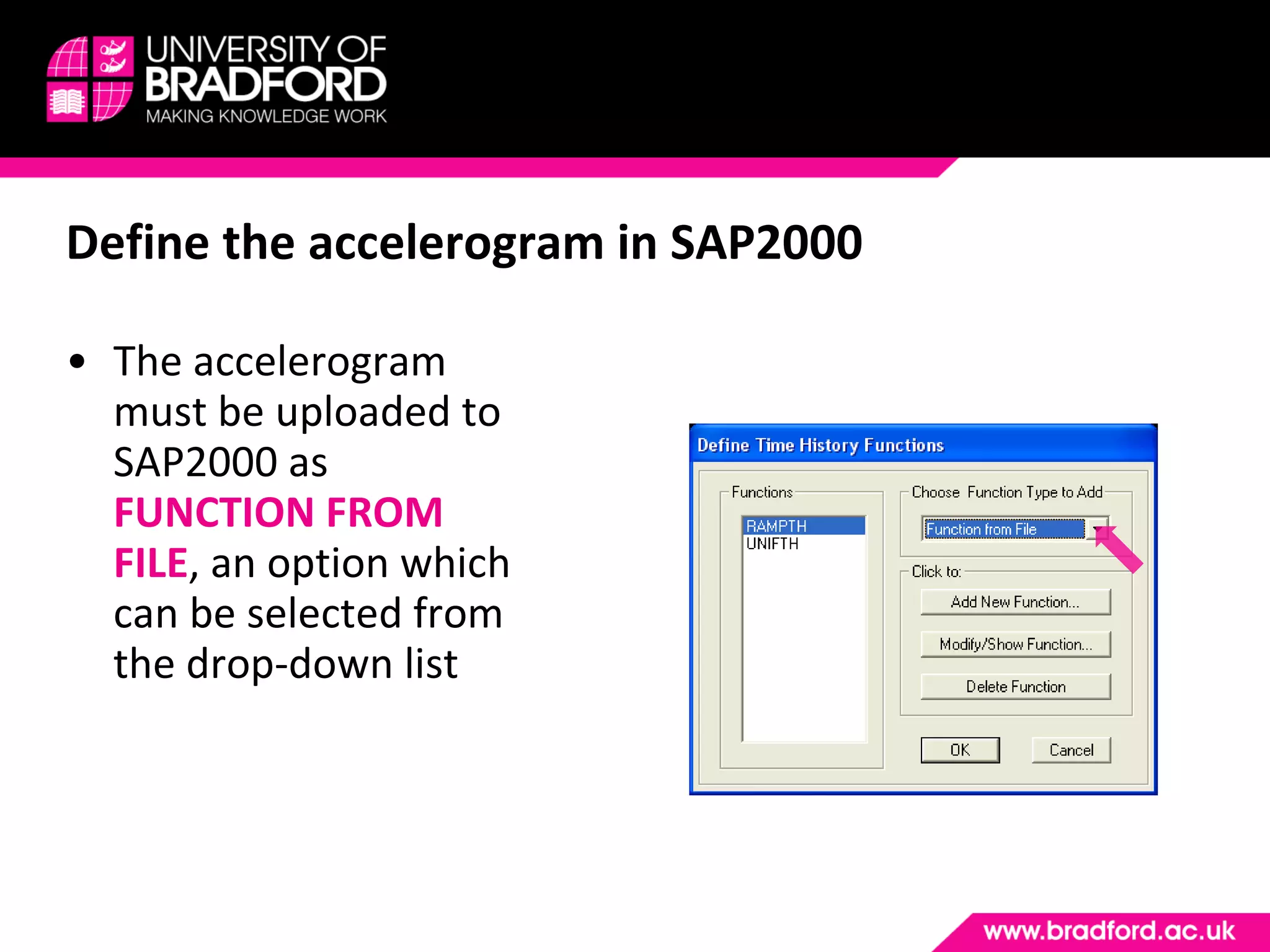
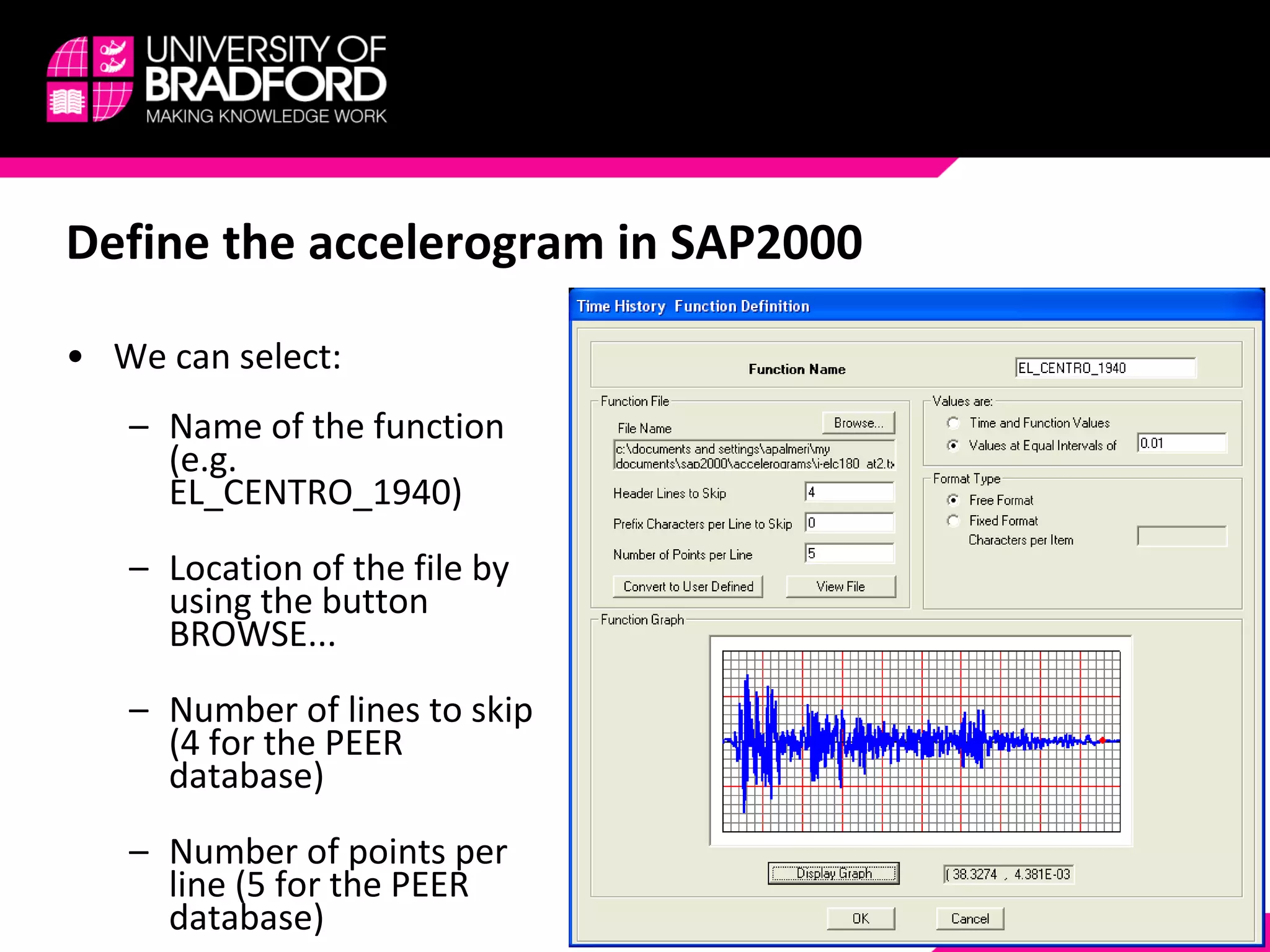
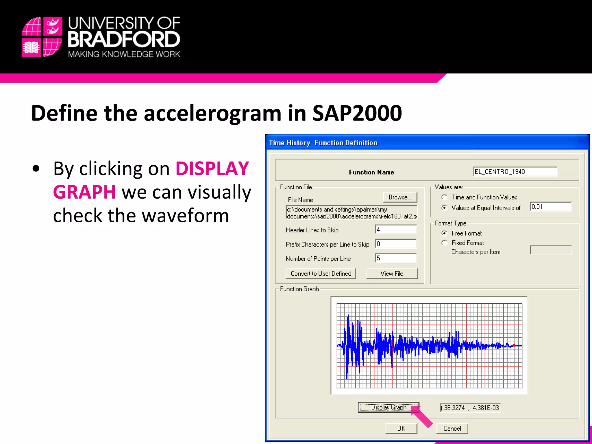
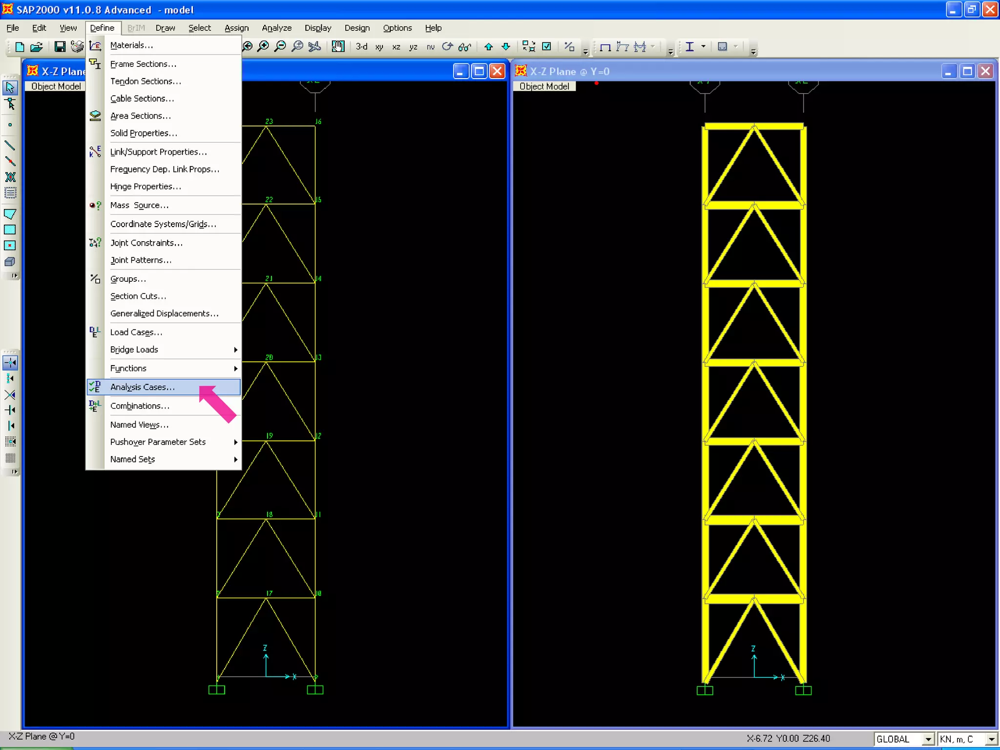
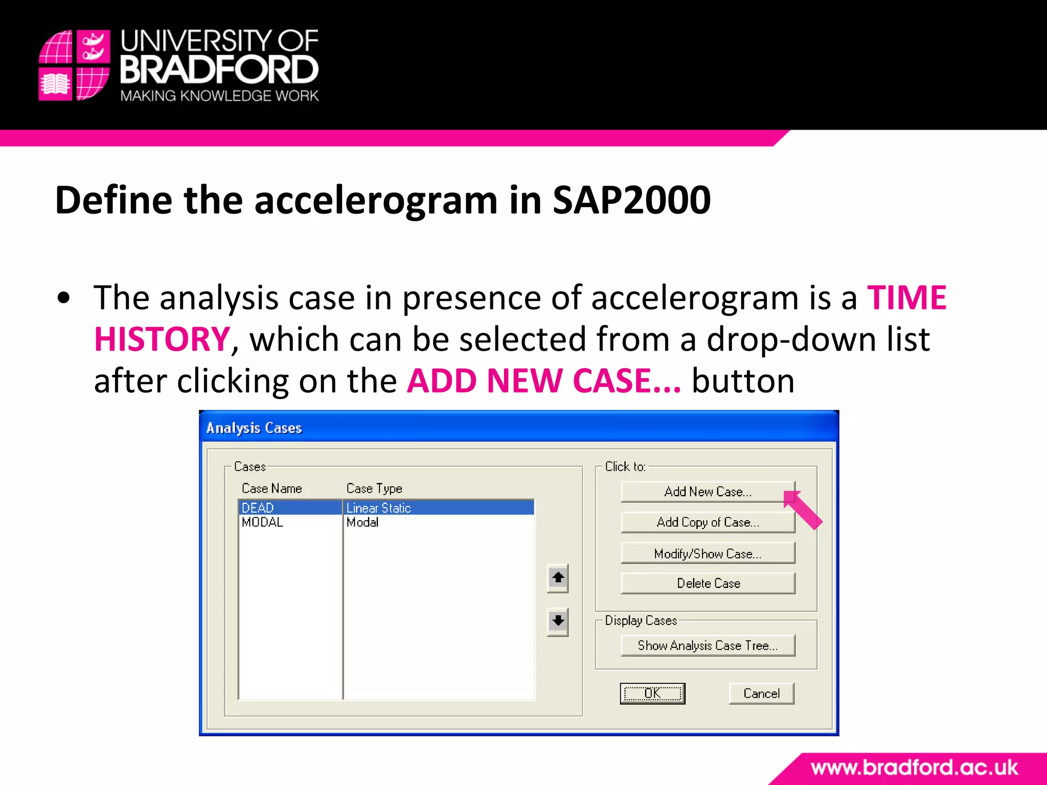
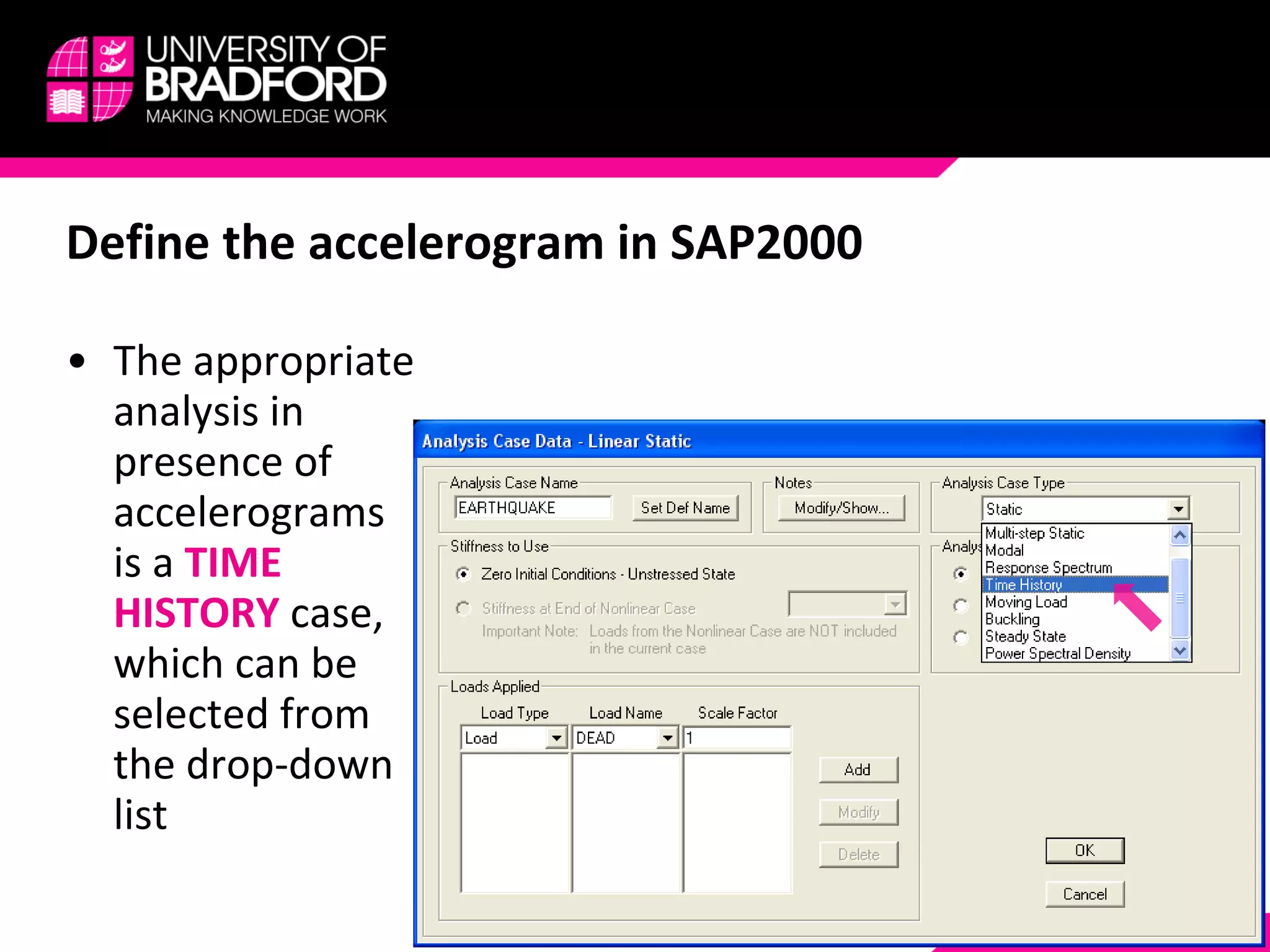
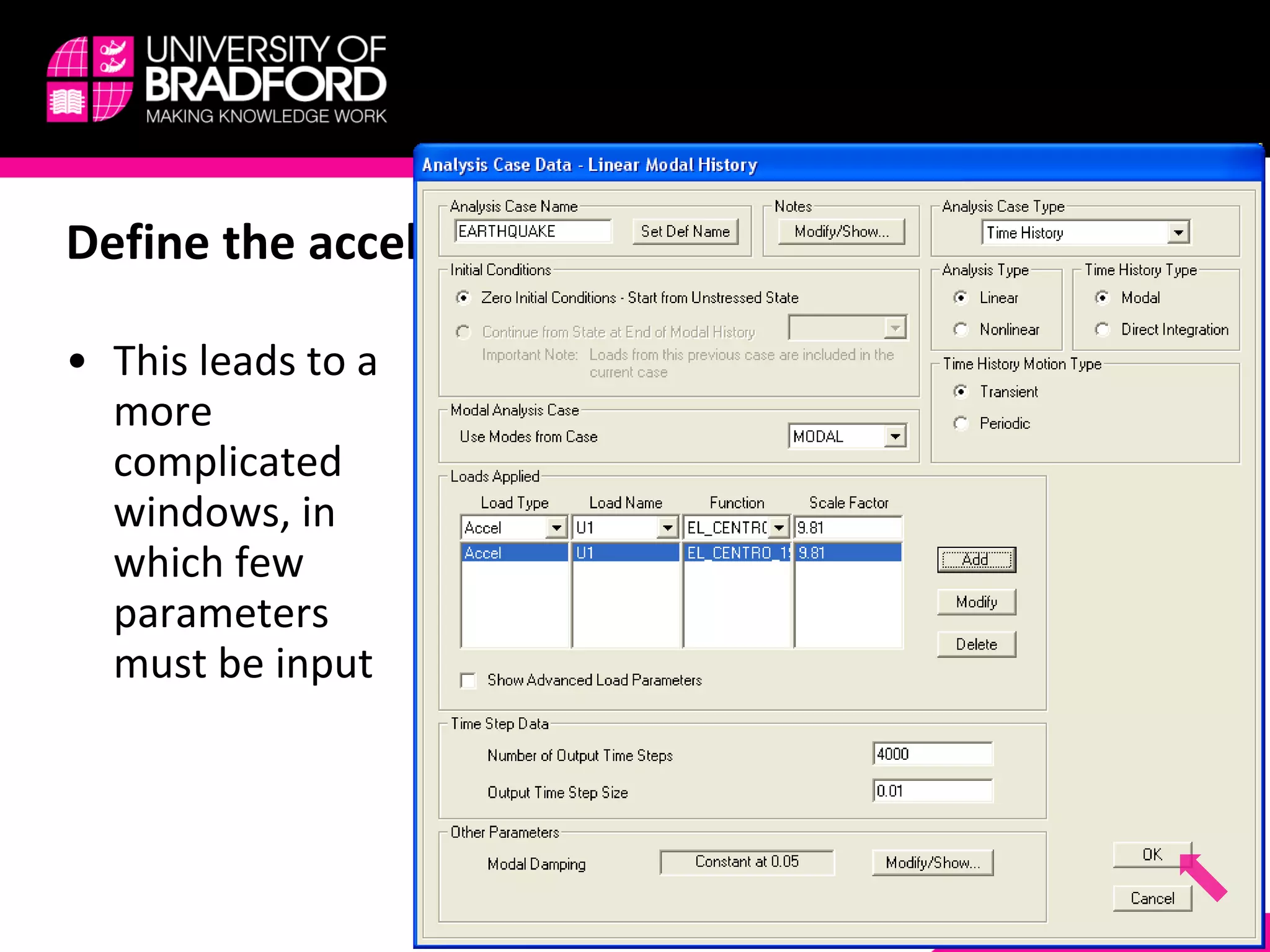
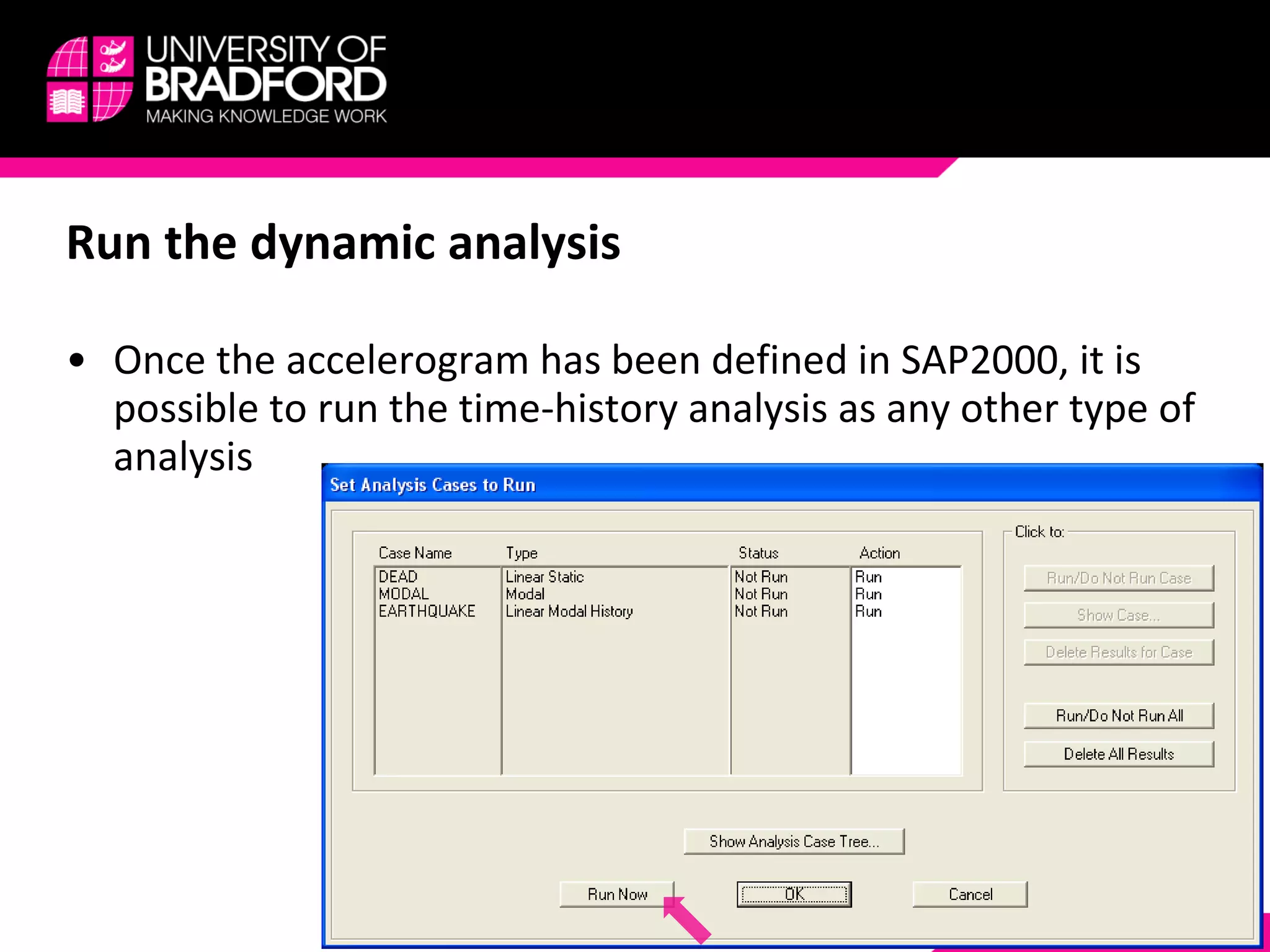
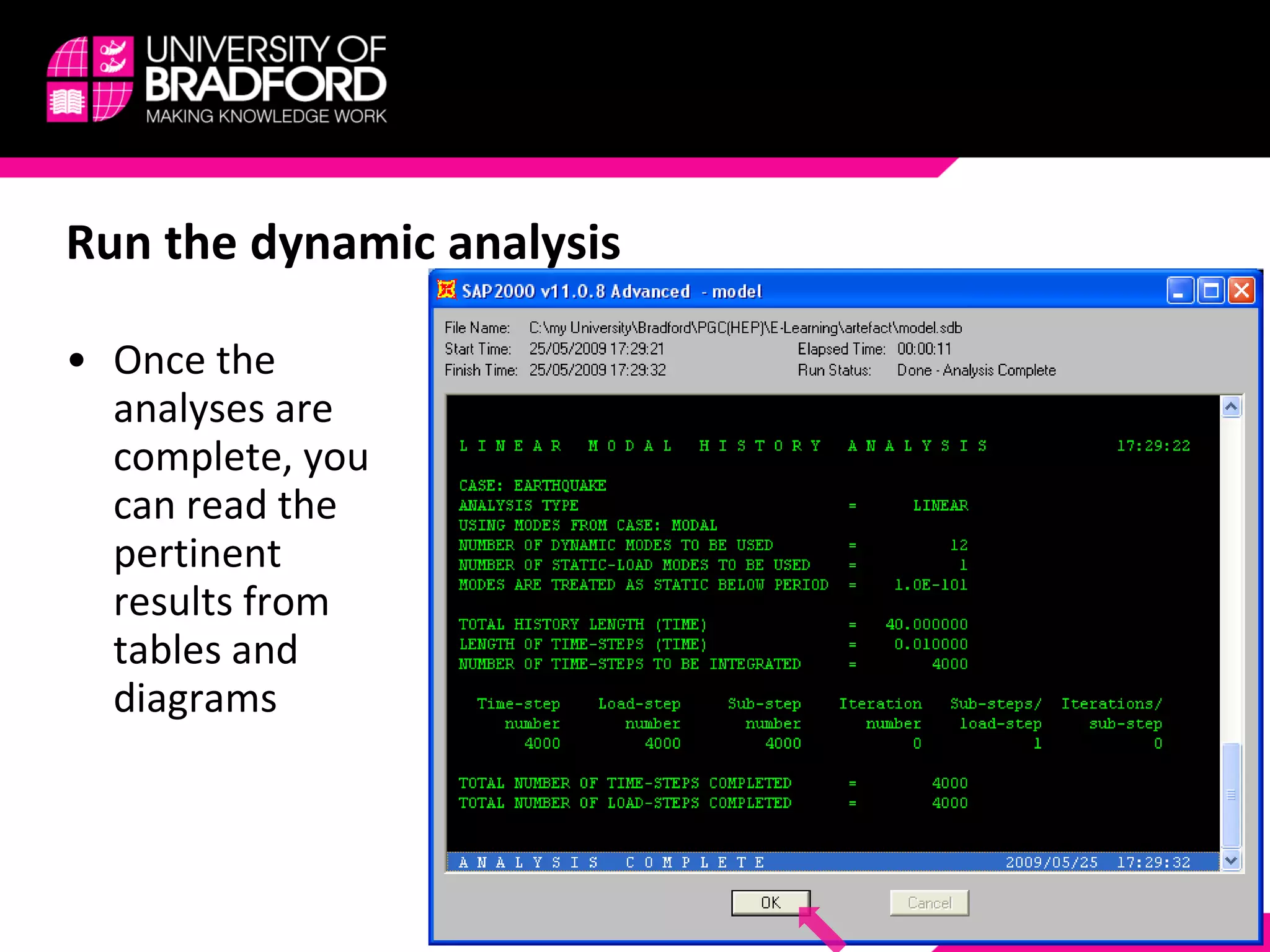
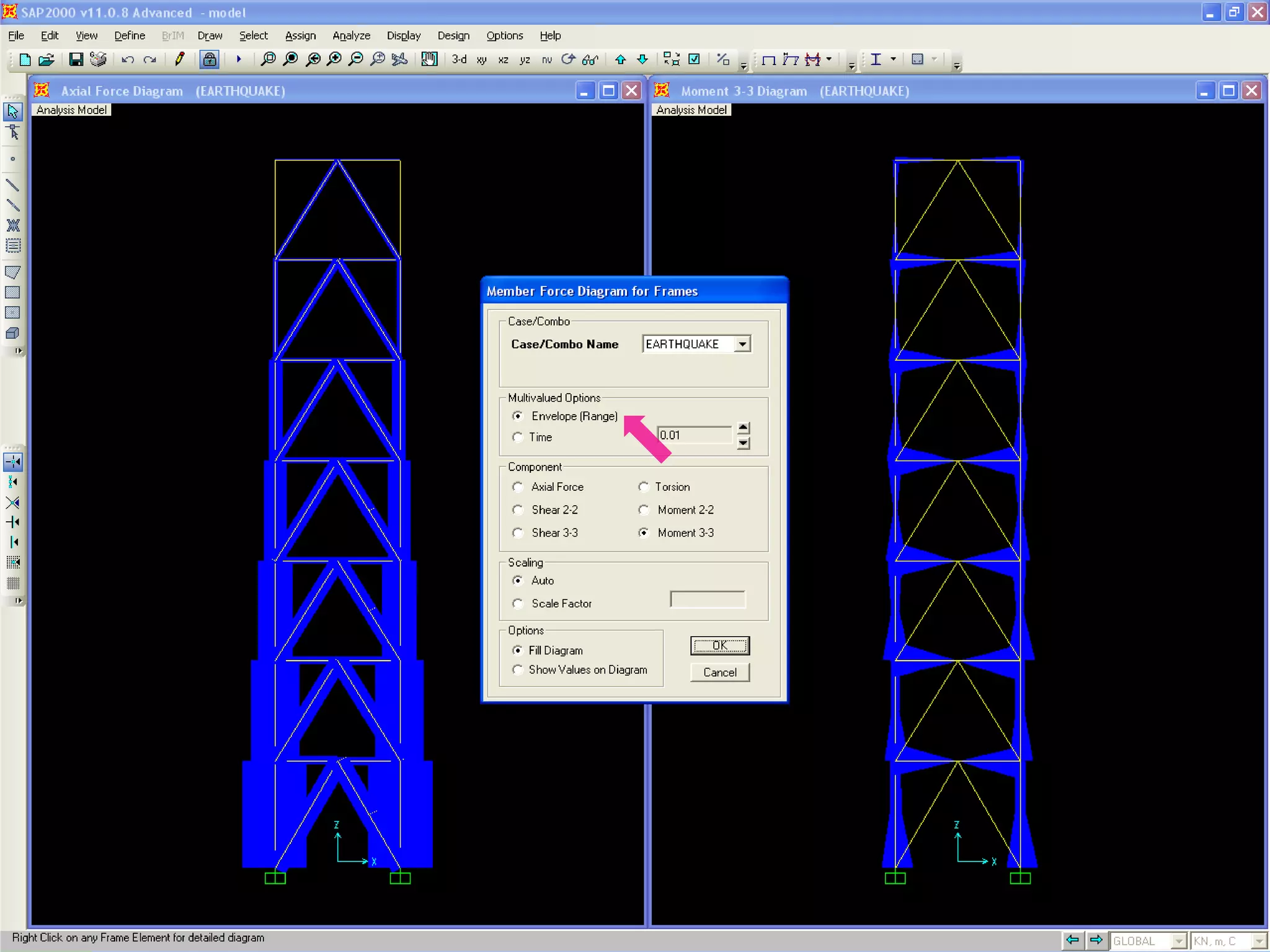
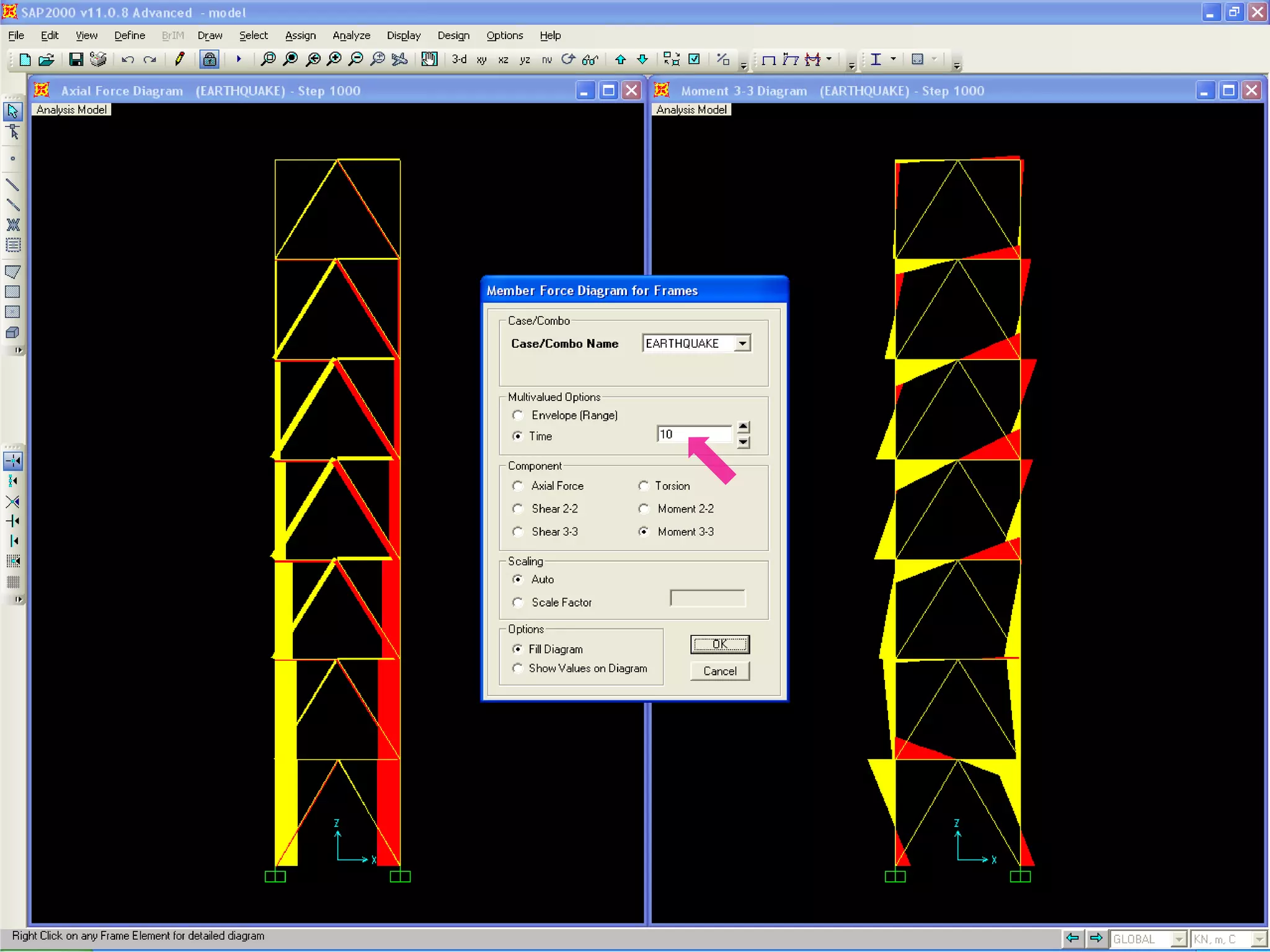
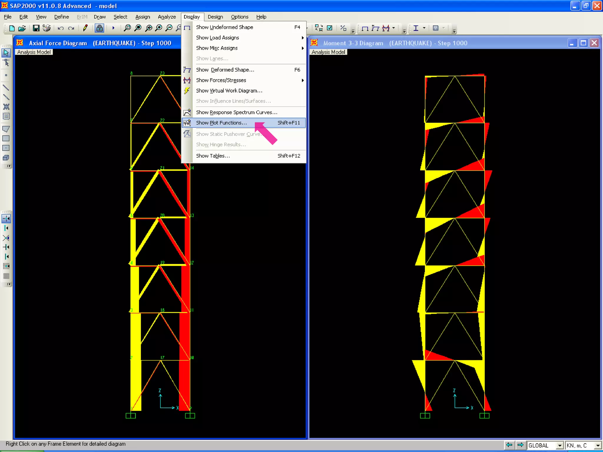
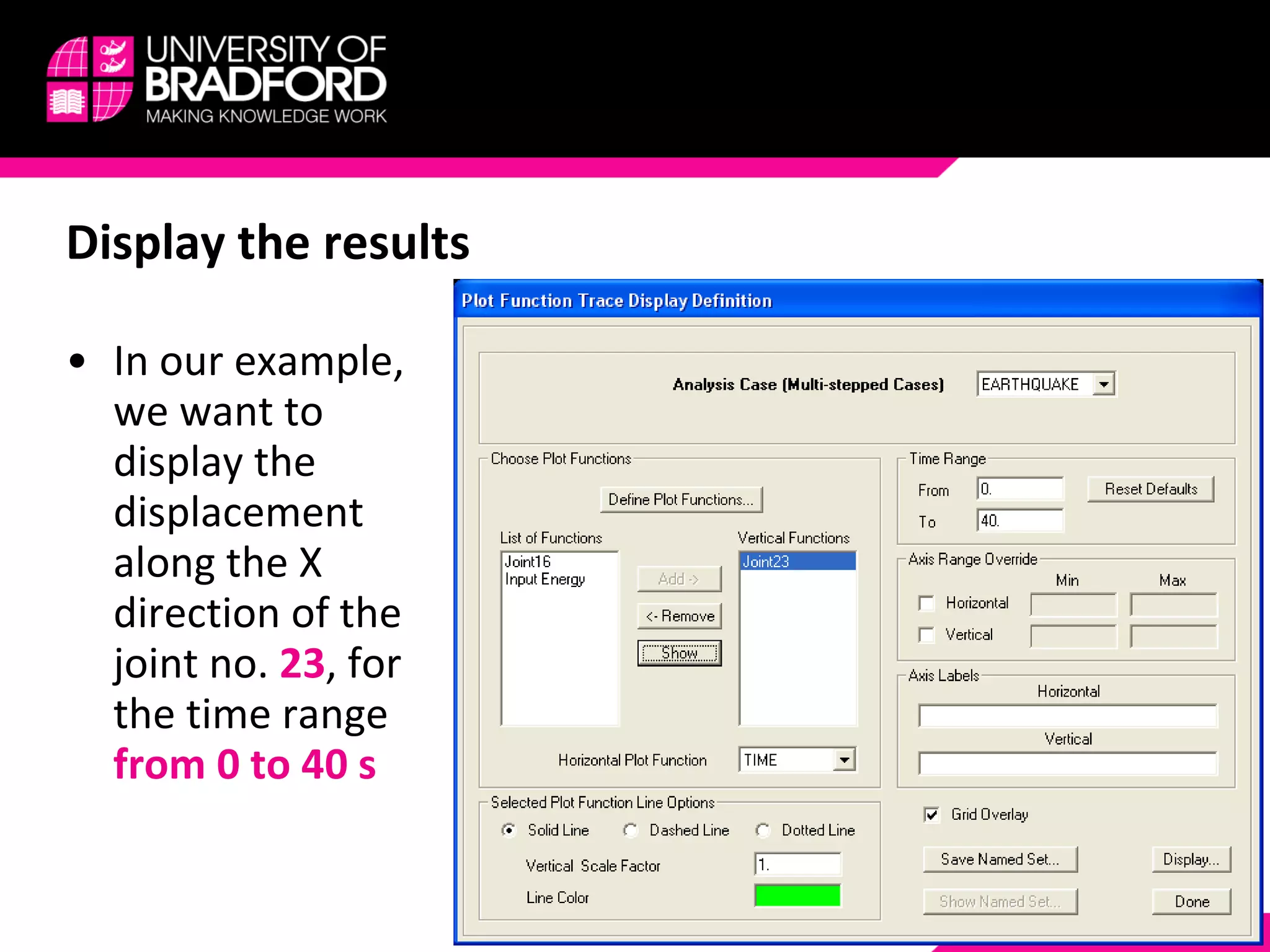
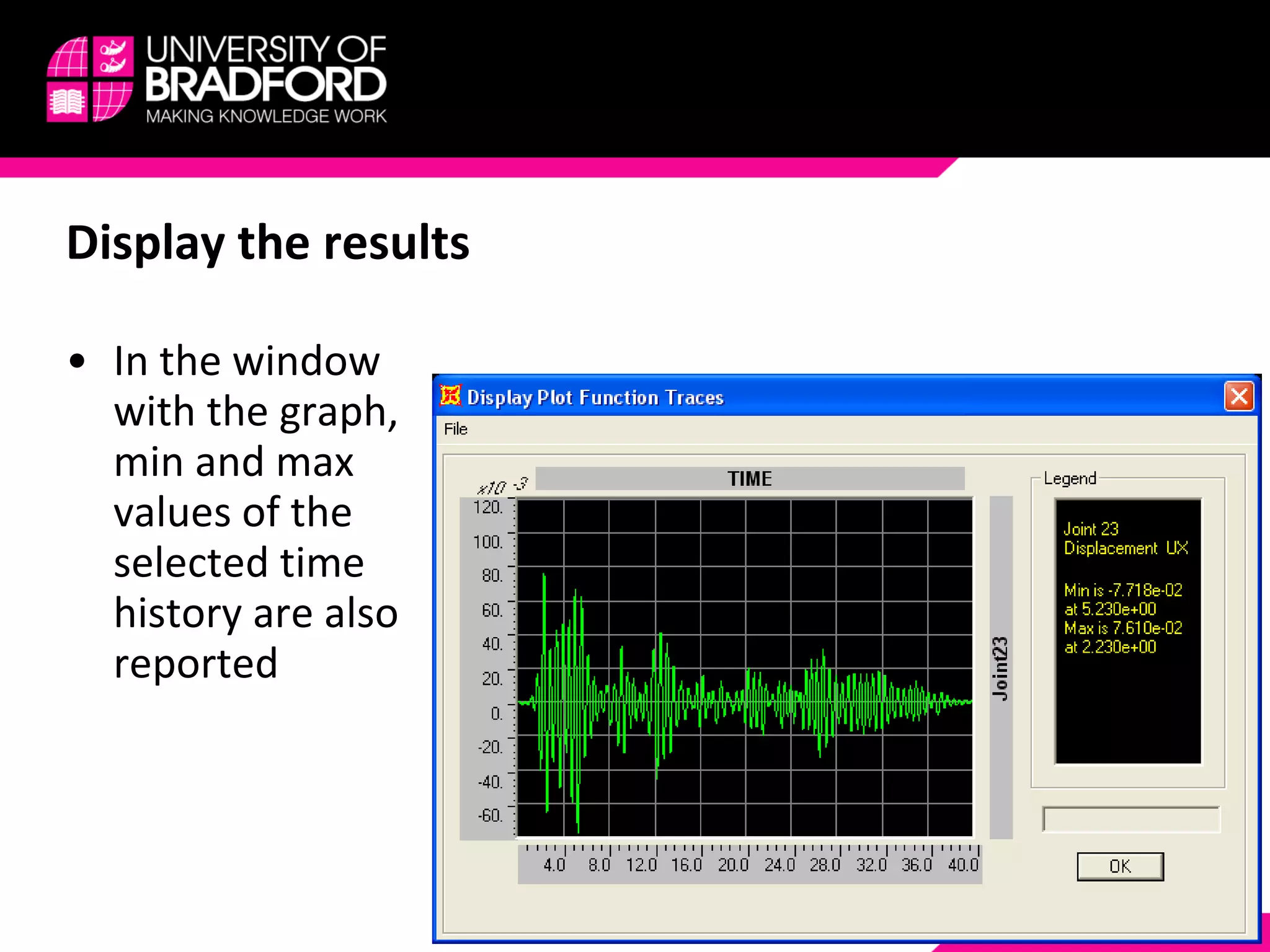
The document provides a step-by-step guide for conducting a time-history seismic analysis using SAP2000 software. It details how to: 1) Download recorded earthquake accelerograms from the PEER database, such as one from the 1940 Imperial Valley earthquake. 2) Upload the selected accelerogram file into SAP2000 and define it as a time history function. 3) Assign the accelerogram to a time history analysis case and run the dynamic analysis. 4) View and analyze results like envelopes of axial forces, moments, and time histories of displacements.

1. Time-history seismic analysis with SAP2000 A step-by-step guide for BEng/MEng/MSc students familiarizing with this piece of software

2. List of Content Download recorded accelerograms from the PEER database Upload a selected accelerogram to SAP2000 Run the time-history analysis and display the results

3. DOWNLOAD ACCELEROGRAMS FROM THE PEER DATABASE Step #1

4. PEER Strong Ground Motion Database The P acific E arthquake E ngineering R esearch (PEER), headquartered at the University of California at Berkeley , makes available online over 10,000 strong ground motion records from 173 different earthquakes http://peer.berkeley.edu/

5. PEER Strong Ground Motion Database The database in entirely searchable http://peer.berkeley.edu/nga/ As an example, we want to download the accelerogram recorded during the Imperial Valley 1940 earthquake Once the event has been selected in the top drop-down list, we must specify to DISPLAY the results “In Table” rather than “On Map” Then we can SEARCH

7. Find the accelerogram By right-clicking on the appropriate record (NGA0006 in our case), a new page is shown with all the relevant pieces of information about this seismic event If we scroll down, the links to the three components of the accelerogram (180°, 270° and vertical) appear

9. Download the time history of the ground acceleration By right-clicking on one of these links (e.g. the first horizontal component, denote with IMPVALL/I-ELC180), a new textual page is opened with the corresponding time history of the ground acceleration

10. The first four lines contain general pieces of information about the record, namely: Location: “Imperial Valley” Date: 19 th May 1940 Time: 4:39am Station: “El Centro Array #9” Direction: Horizontal, 180° Units of acceleration: g= 9.81 m/s 2 (acceleration of gravity) Number of time instants: 4,000 Sampling time: Δ t= 0.01 s (f= 100 Hz) Download the time history of the ground acceleration

11. The other lines list the ordinates of the record (in units of g), which must be read from left to right, row by row Download the time history of the ground acceleration

12. Importantly, the web browser (Explorer, Firefox and etcetera) allows to save this page as a TXT file (you may need to manually change the extension) Download the time history of the ground acceleration

13. UPLOAD ACCELEROGRAMS TO SAP2000 Step #2

14. Define the accelerogram in SAP2000 An accelerogram is basically the time-history of the acceleration experienced by the ground in a given direction during a seismic event We need to input the accelerogram as a generic function defined in SAP2000 starting from a TXT file Once the mechanical model of the structural system under investigation has been created, SELECT from the menu bar: DEFINE -> FUNCTIONS -> TIME HISTORIES...

16. Define the accelerogram in SAP2000 The accelerogram must be uploaded to SAP2000 as FUNCTION FROM FILE , an option which can be selected from the drop-down list

17. Define the accelerogram in SAP2000 We can select: Name of the function (e.g. EL_CENTRO_1940) Location of the file by using the button BROWSE... Number of lines to skip (4 for the PEER database) Number of points per line (5 for the PEER database)

18. Define the accelerogram in SAP2000 By clicking on DISPLAY GRAPH we can visually check the waveform

19. Define the accelerogram in SAP2000 In order to be used in a seismic simulation, the waveform previously defined must be properly assigned to an ANALYSIS CASE To do this, SELECT from the menu bar: DEFINE -> ANALYSIS CASES...

21. Define the accelerogram in SAP2000 The analysis case in presence of accelerogram is a TIME HISTORY , which can be selected from a drop-down list after clicking on the ADD NEW CASE... button

22. Define the accelerogram in SAP2000 The appropriate analysis in presence of accelerograms is a TIME HISTORY case, which can be selected from the drop-down list

23. Define the accelerogram in SAP2000 This leads to a more complicated windows, in which few parameters must be input

24. Define the accelerogram in SAP2000 In particular: The load type is an ACCEL eration of the ground (first drop-down list) For a planar model, the ground shaking is generally assumed to happen in the X direction, i.e. Load name U1 (seconddrop-down list) The records from the PEER website are given in units of g, so the scale factor would be 9.81 m/s 2 or 981 cm/s 2 , depending on the units selected in the model of SAP2000 The number of time steps should be given by the duration of the accelerogram divided by the sampling time: In our example: 40 s / 0.01 s = 4,000 steps

25. RUN THE ANALYSIS AND DISPLAY THE RESULTS Step #3

26. Run the dynamic analysis Once the accelerogram has been defined in SAP2000, it is possible to run the time-history analysis as any other type of analysis

27. Run the dynamic analysis Once the analyses are complete, you can read the pertinent results from tables and diagrams

28. Display the results In the next slides the results of the dynamic analysis are shown in terms of: Axial Force N (left-had side graph) Bending Moment M (right-hand side graph) It is worth mentioning that these blue diagrams are the ENVELOPE of the corresponding outputs: Indeed, in a dynamic analysis we have a value of the structural quantities of interest (e.g. N and M) for each time steps As engineers, we are generally interested in both minimum and maximum value, i.e. by the “envelope” of these responses

30. Display the results We can also display the same structural quantities in a specific time instant, e.g. at t = 10 s ... In this case, for instance, the red colour in the axial-force diagram means compression, while the yellow colour stands for tentions

32. Display the results In order to show the time history of a given structural response, e.g. The horizontal displacement of the top floor, you mus SELECT from the menu bar: DISPLAY -> SHOW PLOT FUNCTIONS...

34. Display the results In our example, we want to display the displacement along the X direction of the joint no. 23 , for the time range from 0 to 40 s

35. Display the results In the window with the graph, min and max values of the selected time history are also reported