Downloaded 2,855 times

![17
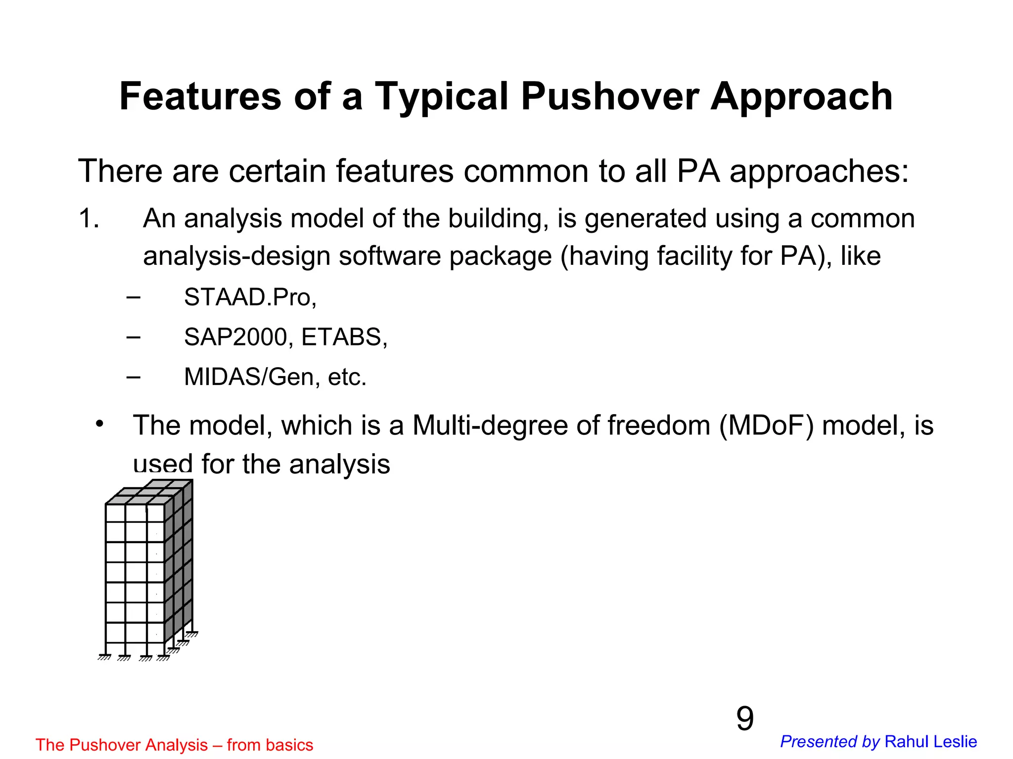
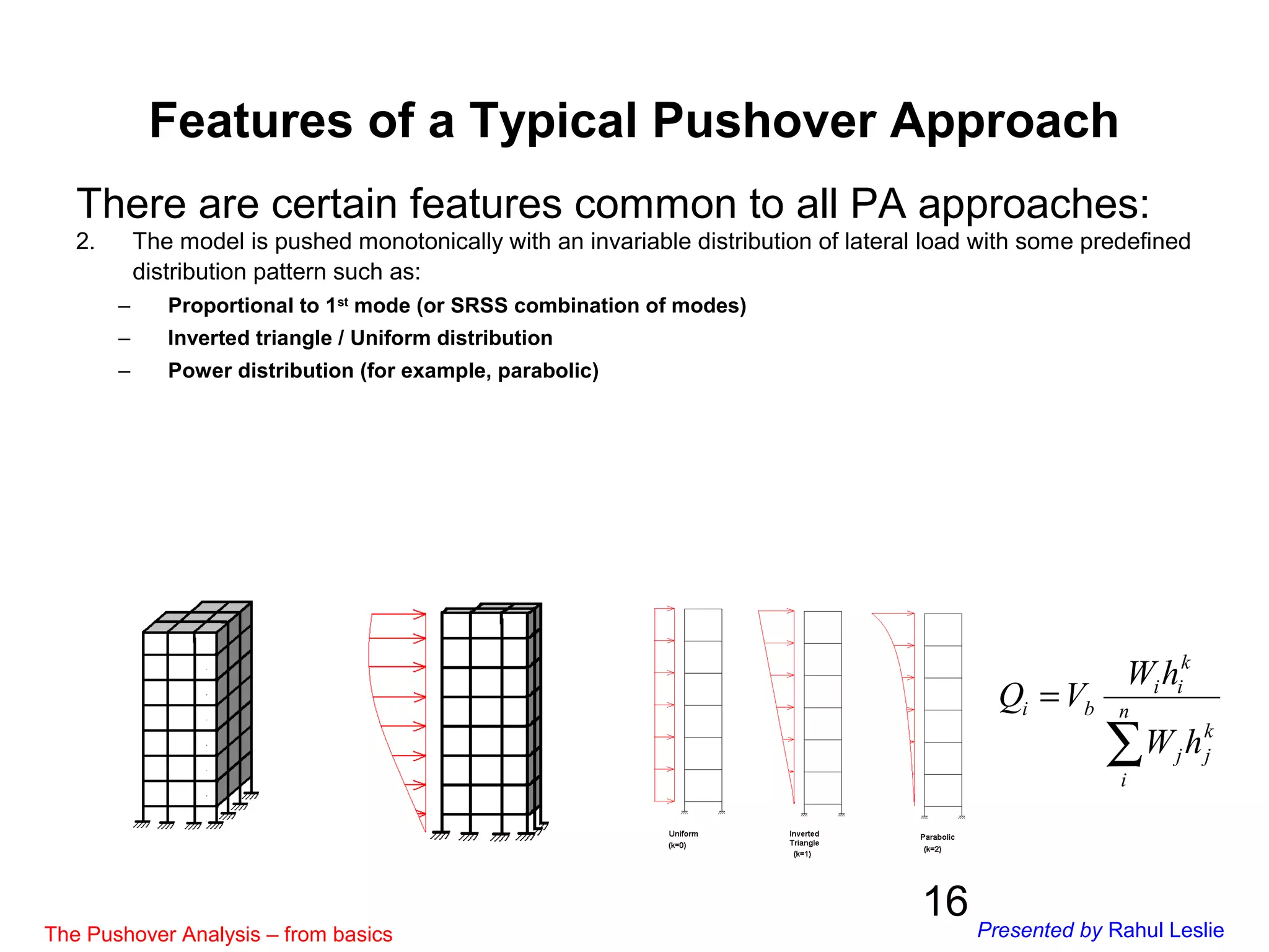
There are certain features common to all PA approaches:
2. (Continuation …)
• Unlike conventional SA, in Pushover analysis, analysis for Gravity
loads is done first, continued by an analysis for Lateral loads.
• Since PA is done to simulate the behaviour under actual loads, the
Gravity loads applied are not factored, but in accordance with
Cl.7.3.3 and Table 8 of IS:1893-2002 :
[DL + 0.25 LL≤3kN/sq.m + 0.5 LL>3kN/sq.m]
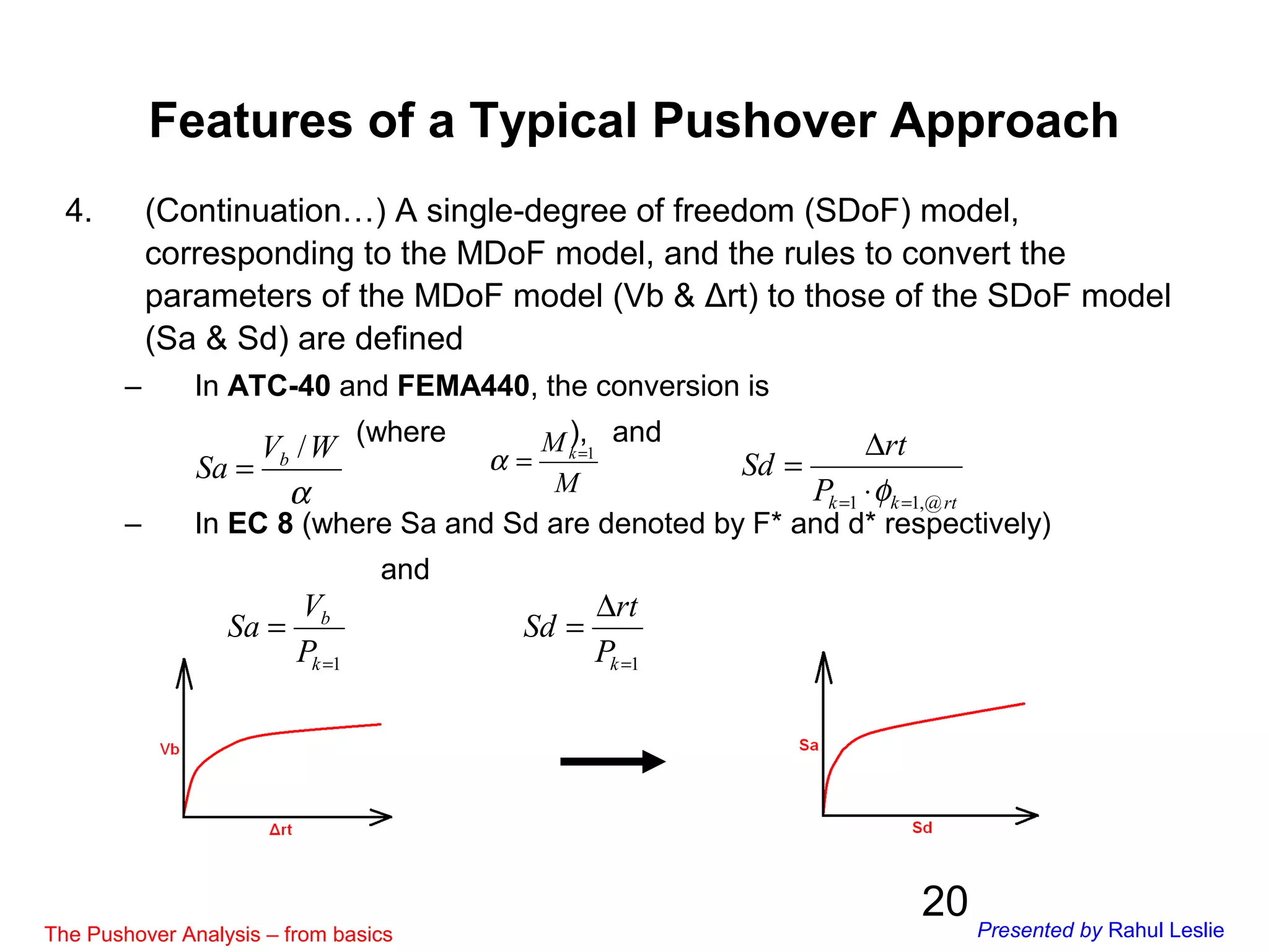
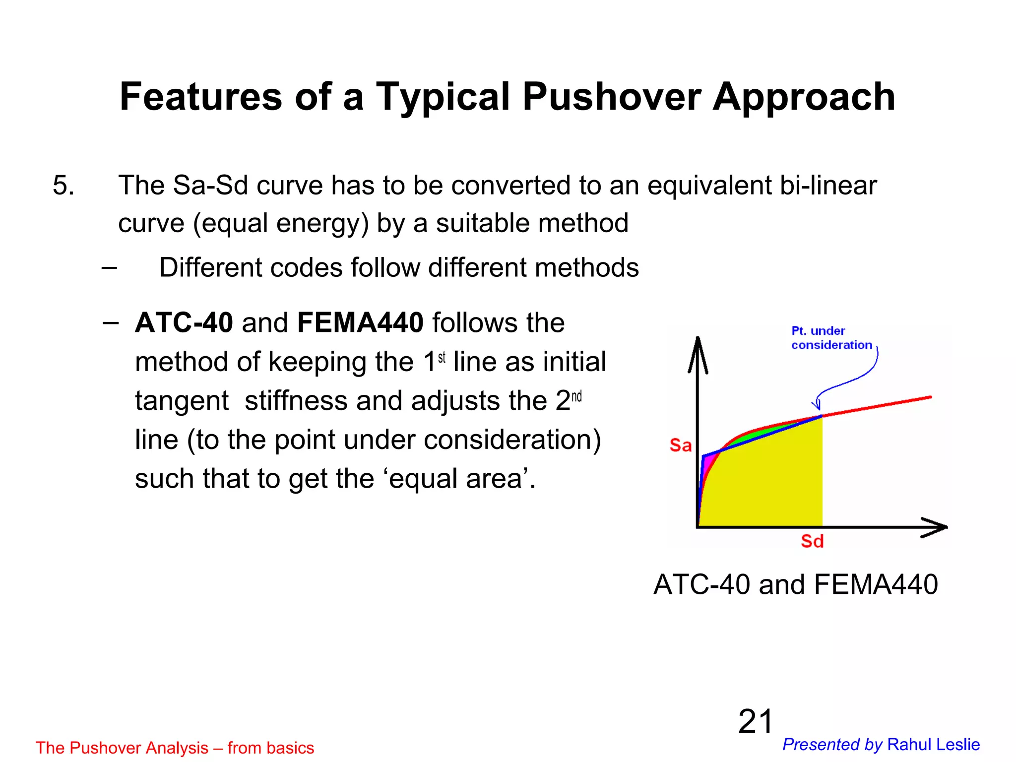
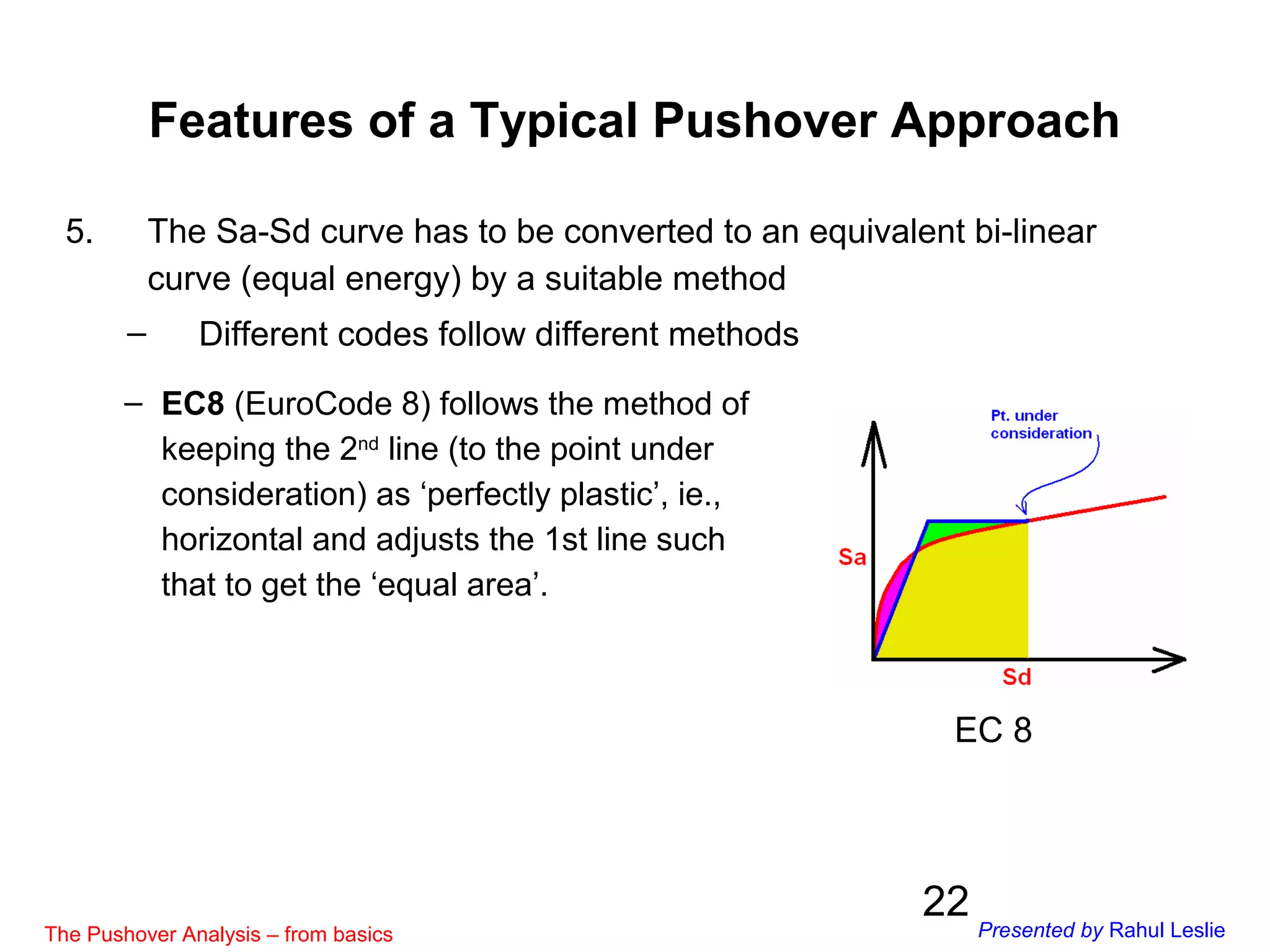
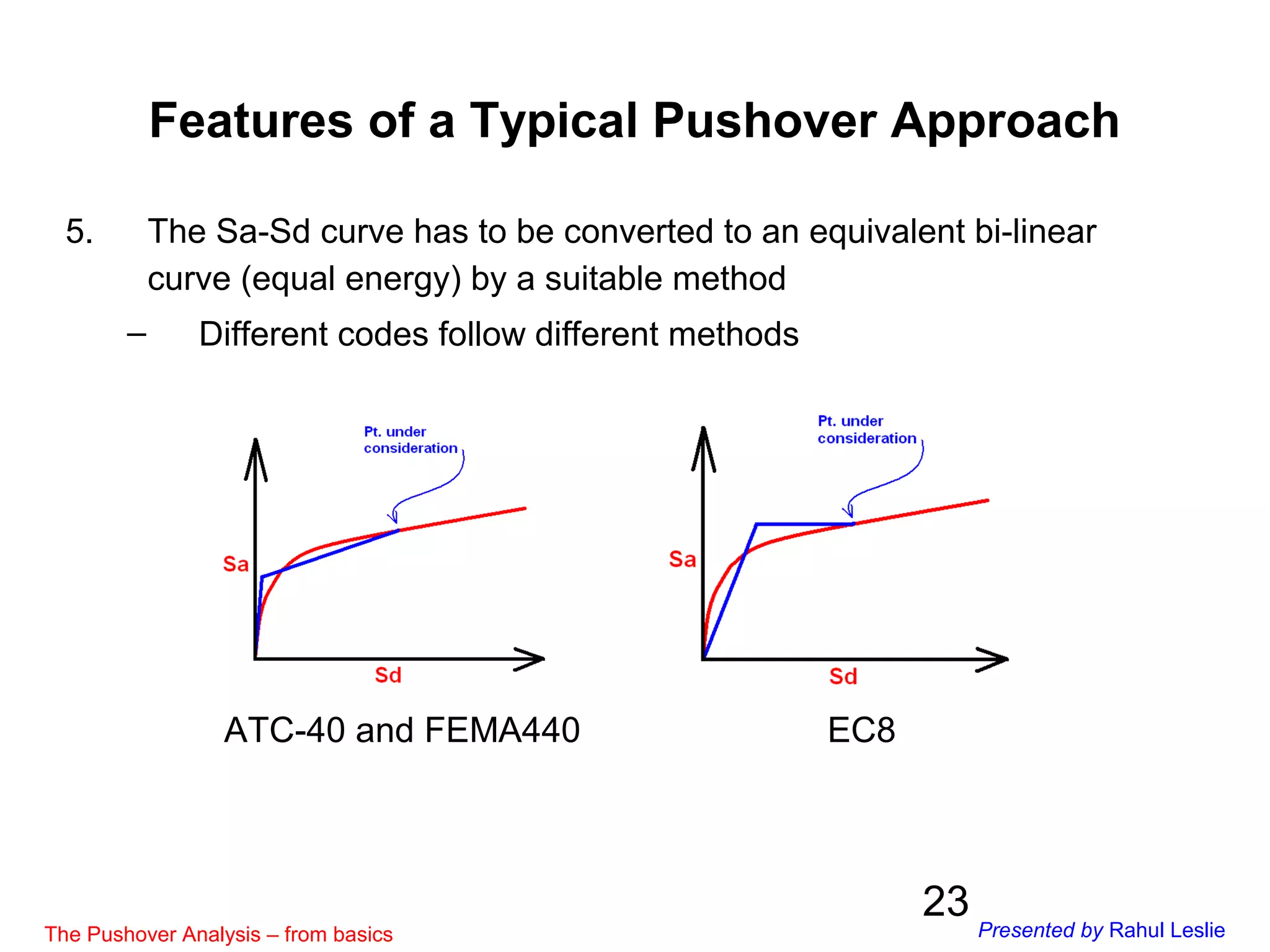
Features of a Typical Pushover Approach
The Pushover Analysis – from basics Presented by Rahul Leslie](https://image.slidesharecdn.com/pushoveranalysisfrombasicsrahulleslie080216-160213015605/75/The-Pushover-Analysis-from-basics-Rahul-Leslie-17-2048.jpg)


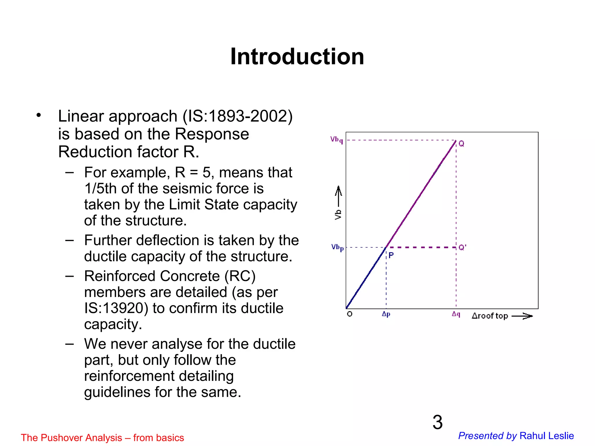
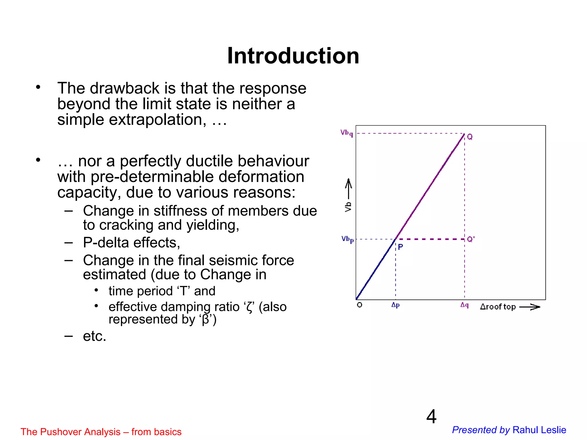
The document presents an overview of pushover analysis (PA), a non-linear static analysis procedure for evaluating a building's strength capacity beyond its limit state during seismic events. It highlights the limitations of linear elastic analysis and discusses the methodology for implementing PA, which includes the creation of a multi-degree of freedom (MDOF) model and the use of non-linear hinges to predict progressive failures and identify weak areas. Additionally, the document compares two main approaches in PA—the displacement coefficient method and the capacity spectrum method—along with their respective steps and features.


