Downloaded 68 times
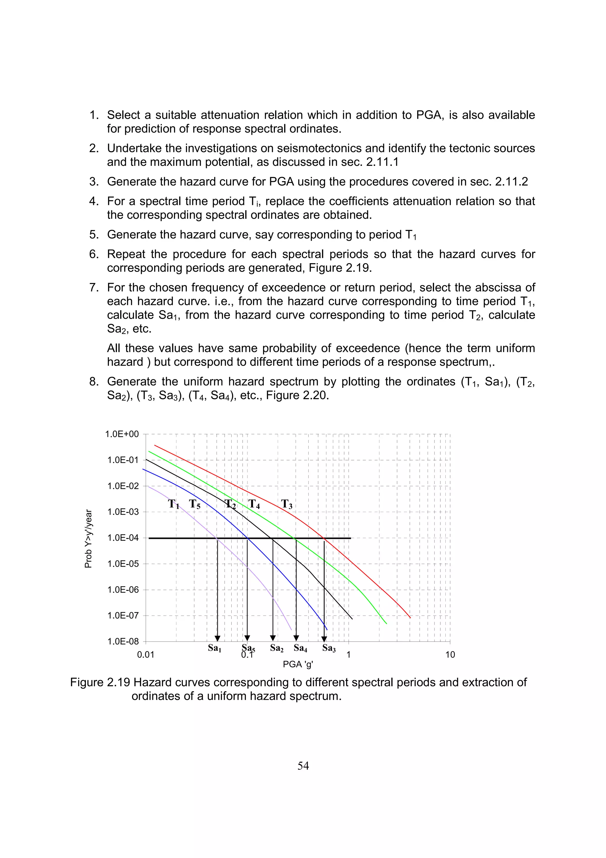
![38
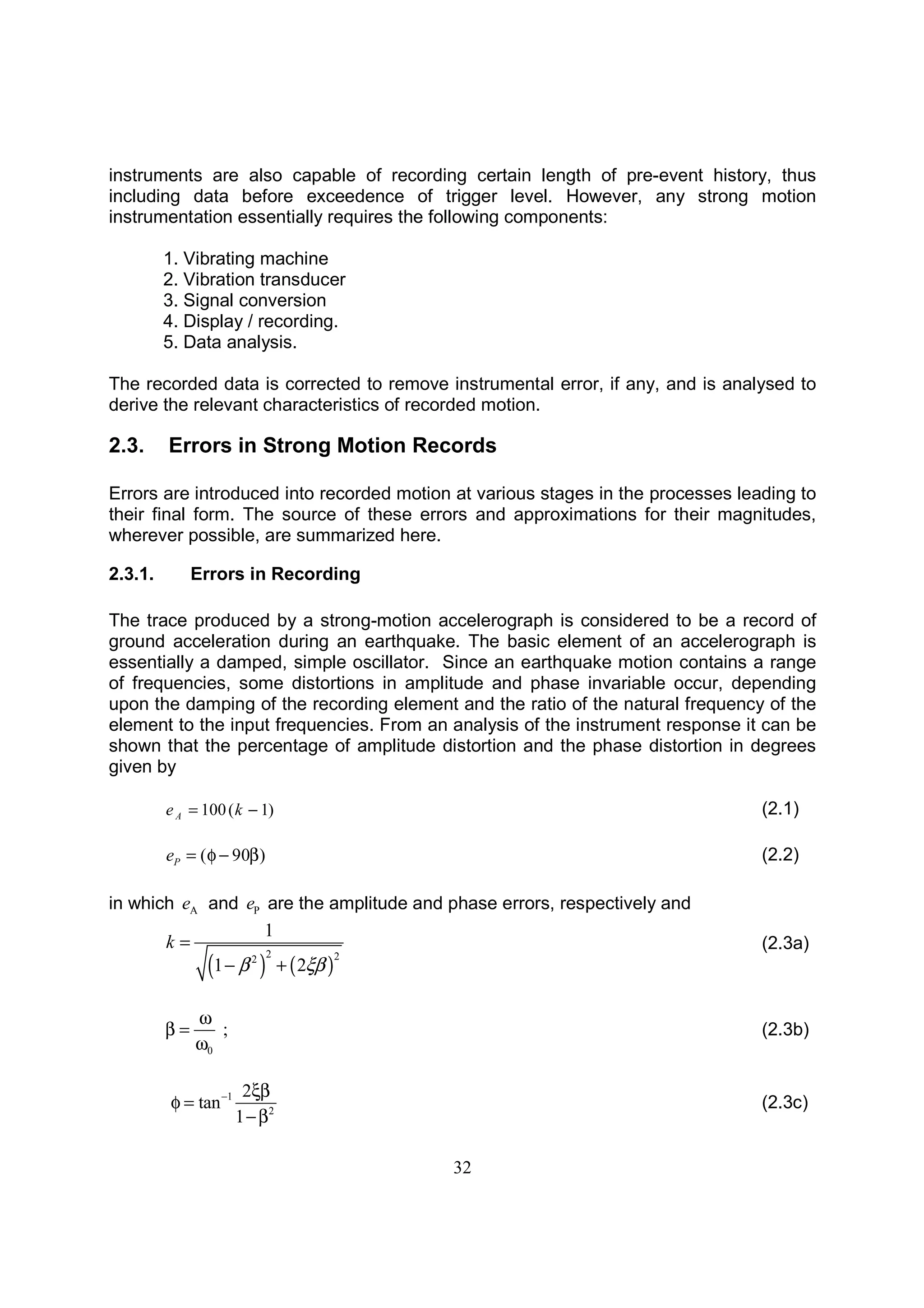
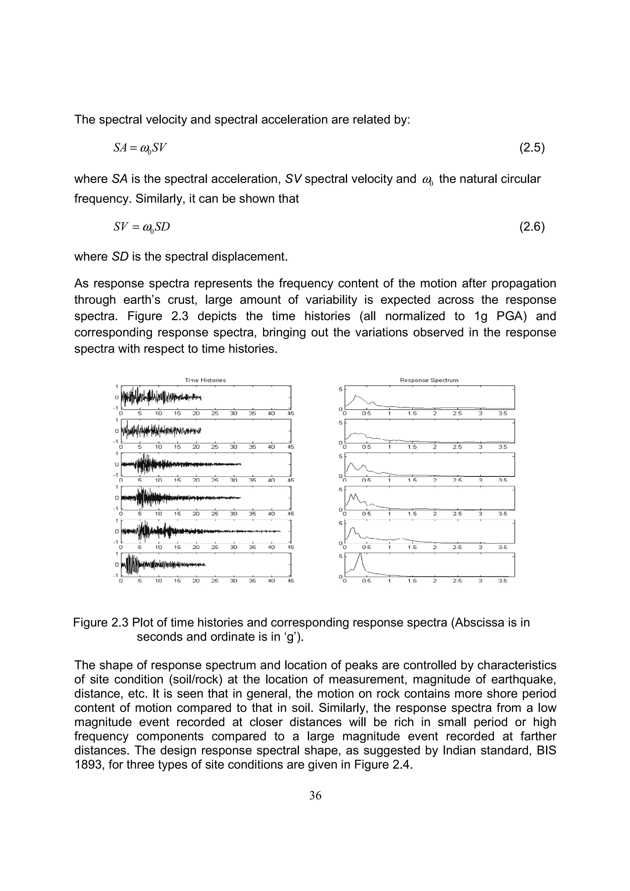
Figure 2.5 A typical tripartite plot or DVA spectrum (From Datta, 2010).
Based on this information, a three zone model of the tripartite plot can be postulated.
These are a displacement sensitive region (that is, long period region), an acceleration
sensitive region (that is, the short period region), and a velocity sensitive region (that is,
the intermediate period region), Figure 2.6. This input is used for estimation of a design
response spectrum from the inputs of peak ground acceleration, peak velocity and peak
displacement.
Figure 2.6 A typical tripartite plot of response spectrum magnifying the constant
acceleration, velocity and displacement regions [From Datta, 2010].](https://image.slidesharecdn.com/02chapter-160115132216/75/02-chapter-Earthquake-Strong-Motion-and-Estimation-of-Seismic-Hazard-9-2048.jpg)
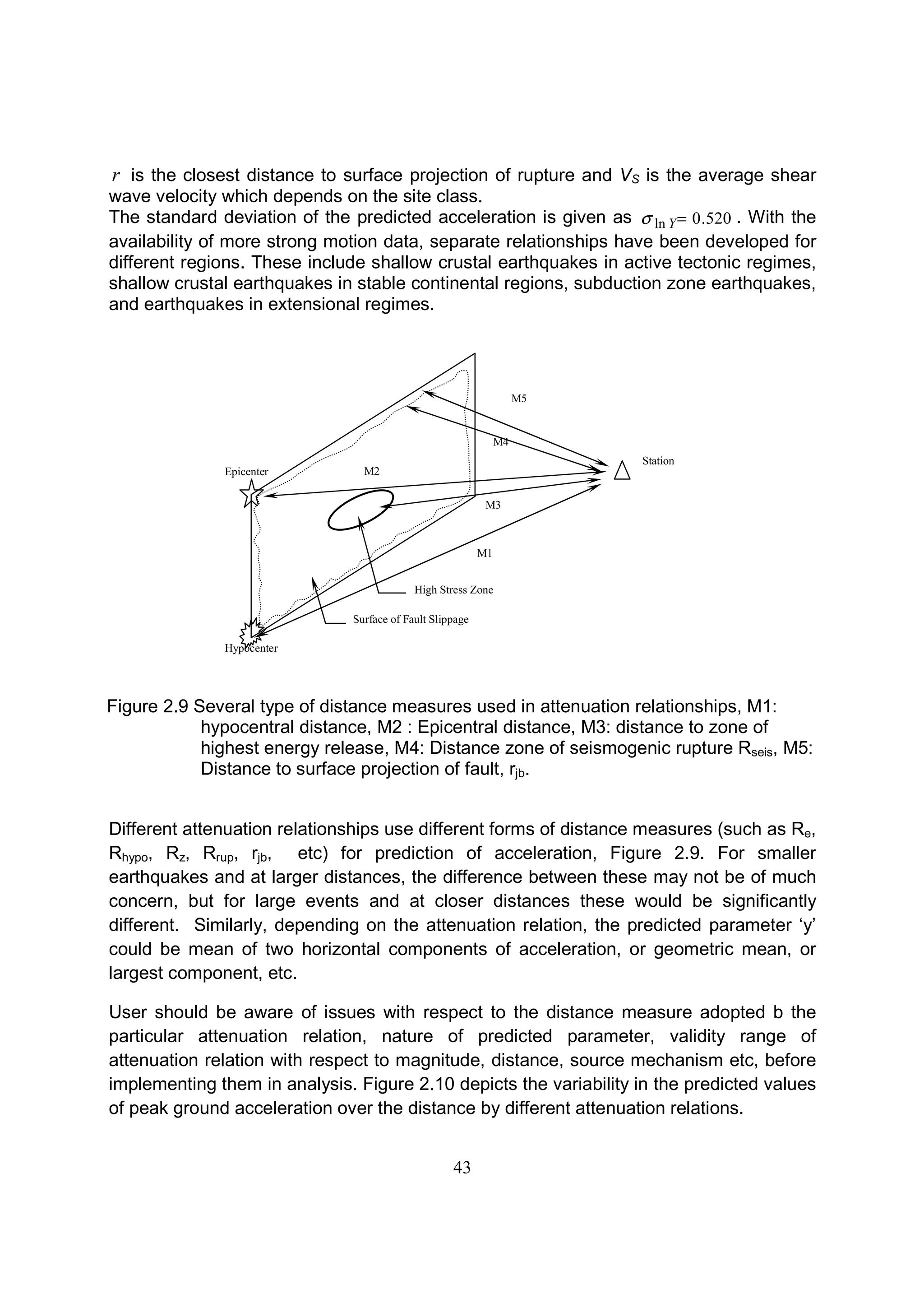
![42
attenuation relationships developed are constantly updated based on the availability of
new data for the particular region.
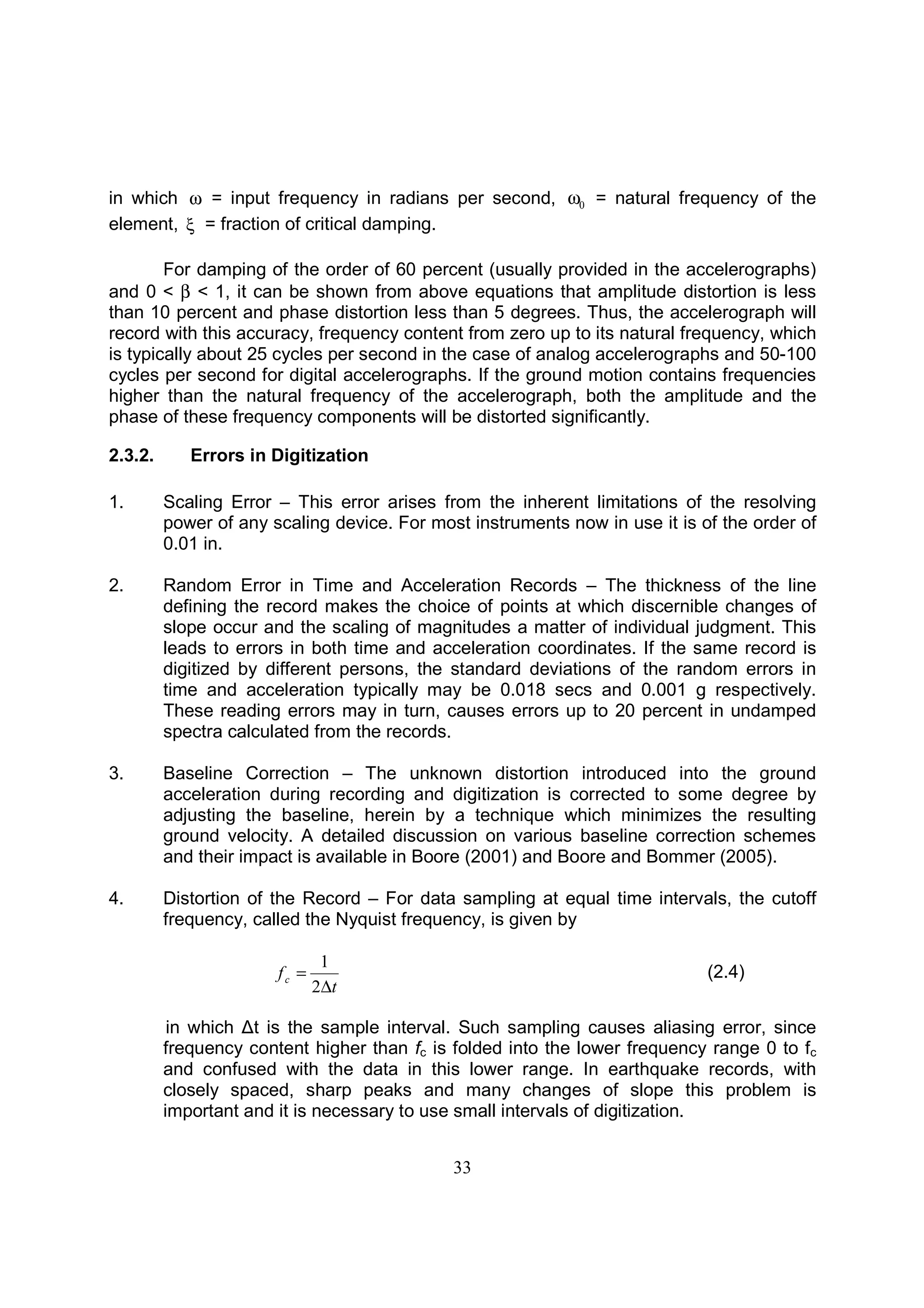
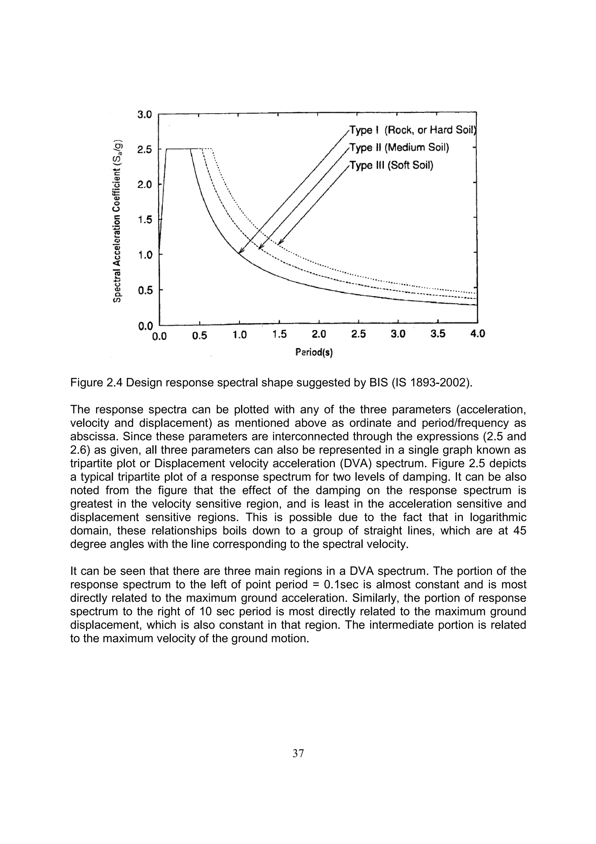
2.9.1. Predictive Relationships for PGA
The acceleration produced by an earthquake is a function of earthquake magnitude and
distance from the source. The attenuation of ground motion is represented by
attenuation relationships. Generally, these empirical relationships have the following
form:
RCmCCLn(y) 321 −+= (2.8)
where ‘m’ is the magnitude of the earthquake and R is the distance from site. C1, C2 and
C3 are constants and are a function of the regional geology and soil conditions. ‘y’ is the
acceleration at site due to earthquake of magnitude ‘m’ occurring at distance R.
In addition to the above terms, recent attenuation relationships also include functions to
account for non linear dependence of attenuation on distance (usually a log (R)
function), site conditions (soft soil, stiff soil, rock, etc), source type and location of
measurement (reverse/strike slip/normal, hanging wall side or foot wall side), etc.
So a more comprehensive form of attenuation relation would be of the type:
[ ] ( ) ( )sourcefCeffectssitefCRCeCRCmCmCCy mCc
109865321 _ln)ln( 74
+++++++=
(2.9)
The coefficients of the equation are determined from observed data using regression
techniques, which uses minimization of error between the measured and predicted
values to calculate the coefficients. Because of this, the predicted value of parameter
would represent a mean estimate with an associated value of standard deviation. It can
be seen from the equation that the acceleration is directly proportional to magnitude and
inversely proportional to distance. Hence, for estimating the maximum acceleration at a
site, one needs to estimate the upper limit magnitude and lower limit of distance.
The attenuation relation for peak ground acceleration (in terms of g) for shallow crustal
earthquakes, as reported by Boore et. al. (1997), is given by
1396
ln371.0ln778.0)6(527.0ln 1
SV
rMbY −−−+= (2.10)
where
−
−−
−−
=
specifiednotismechanismif242.0
faultsslipreversefor117.0
faultsslipstrikefor313.0
1b](https://image.slidesharecdn.com/02chapter-160115132216/75/02-chapter-Earthquake-Strong-Motion-and-Estimation-of-Seismic-Hazard-13-2048.jpg)
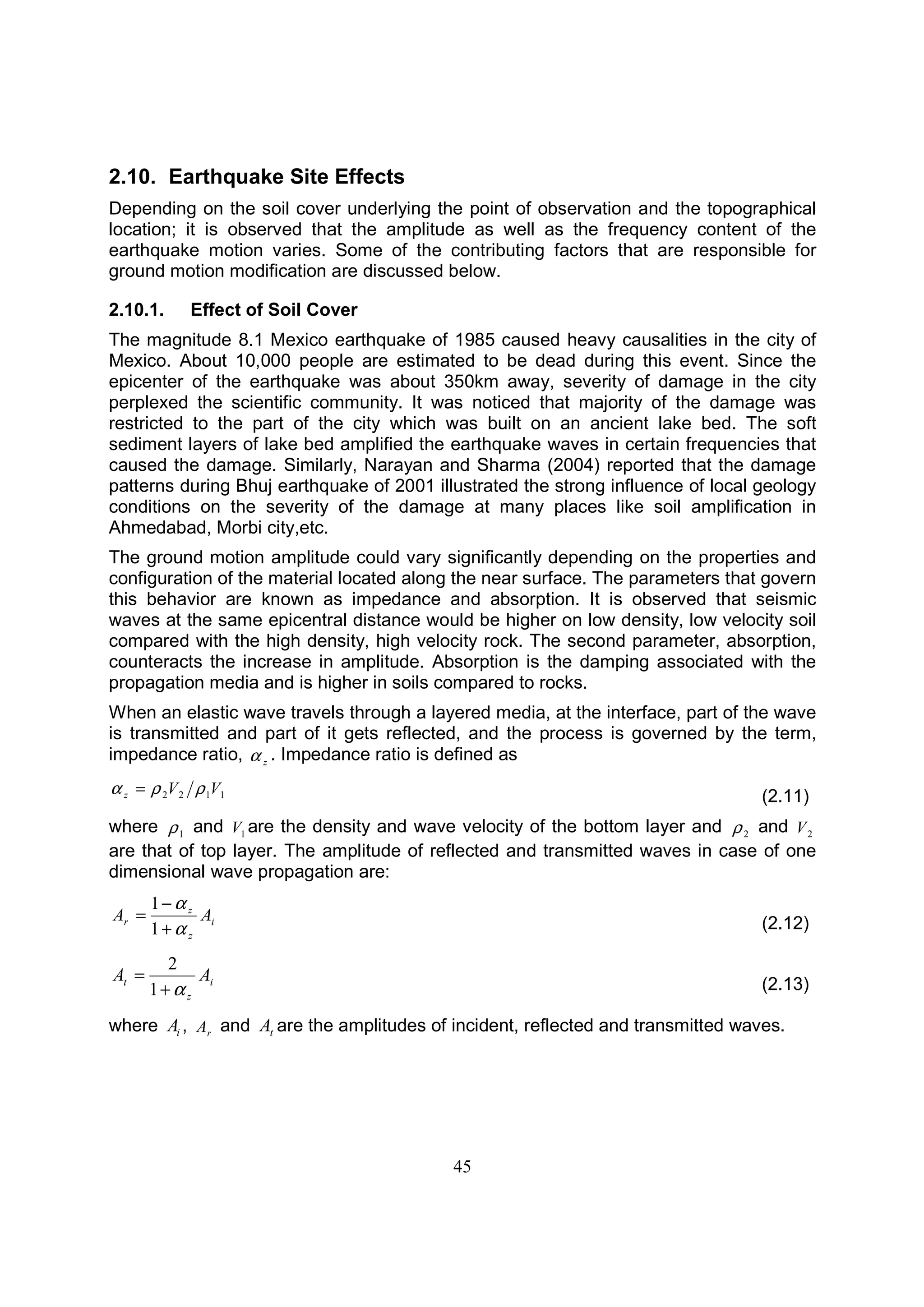
![46
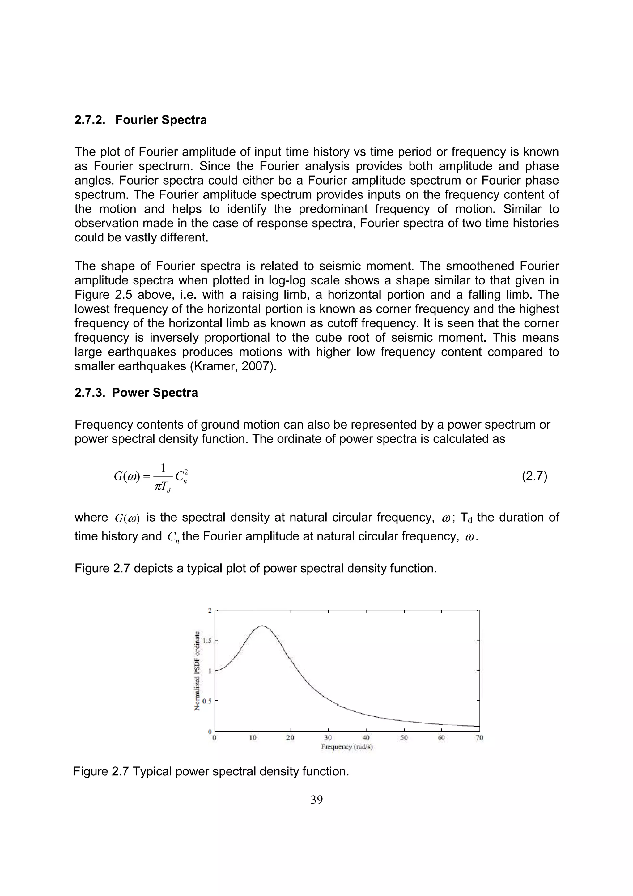
From these, it can be observed that for a value of impedance ration equal to zero, i.e.,
free surface, the amplitude of transmitted wave will be twice that of incident wave.
Similarly, an impedance ratio of 0.25 implies that transmitted wave will have 60% more
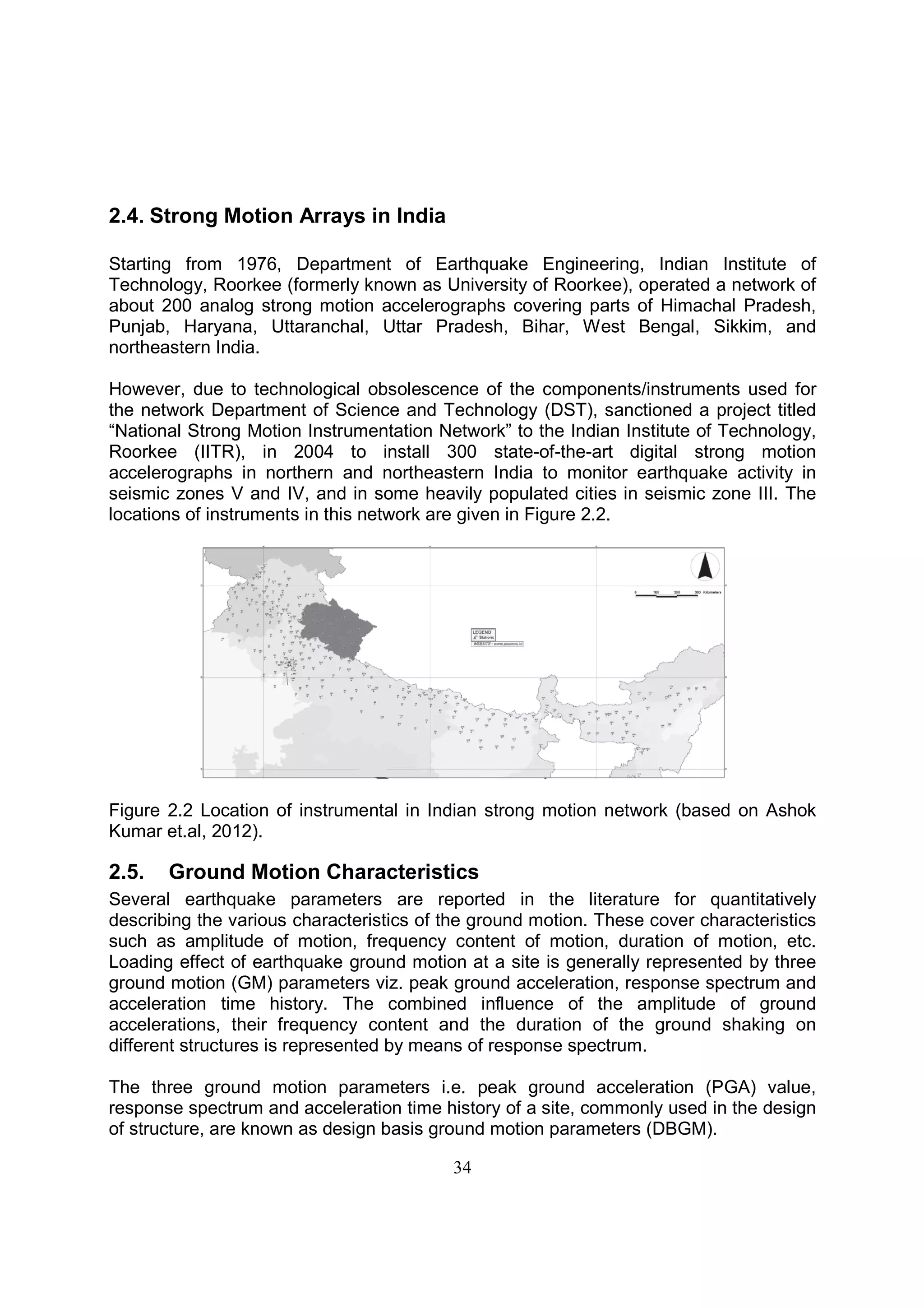
amplitude compared with incident wave. A comparison of the peak ground accelerations
estimated in soil sites viz-a-viz that in rock sites are given in Figure 2.12. It is noted that
the site conditions effects not only the peak acceleration at the site, but also the
frequency content of the motion. The deeper soil layer is found to shift the predominant
period of the ground motion into the longer periods. But the amount of amplification or
de-amplification shift depends on the depth of soil layer and the related soil properties.
Figure 2.13 depicts the relative amplification of motion with respect to depth of soil
cover.
Figure 2.13 Relative amplificaiton factors for a 5% damped response spectrum for sites
with different depths of overlying soil [From Reiter, 1989].
Figure 2.12 A comparison of ground motions recorded on soil and
rock sites [From Kramer, 2008].](https://image.slidesharecdn.com/02chapter-160115132216/75/02-chapter-Earthquake-Strong-Motion-and-Estimation-of-Seismic-Hazard-17-2048.jpg)
![50
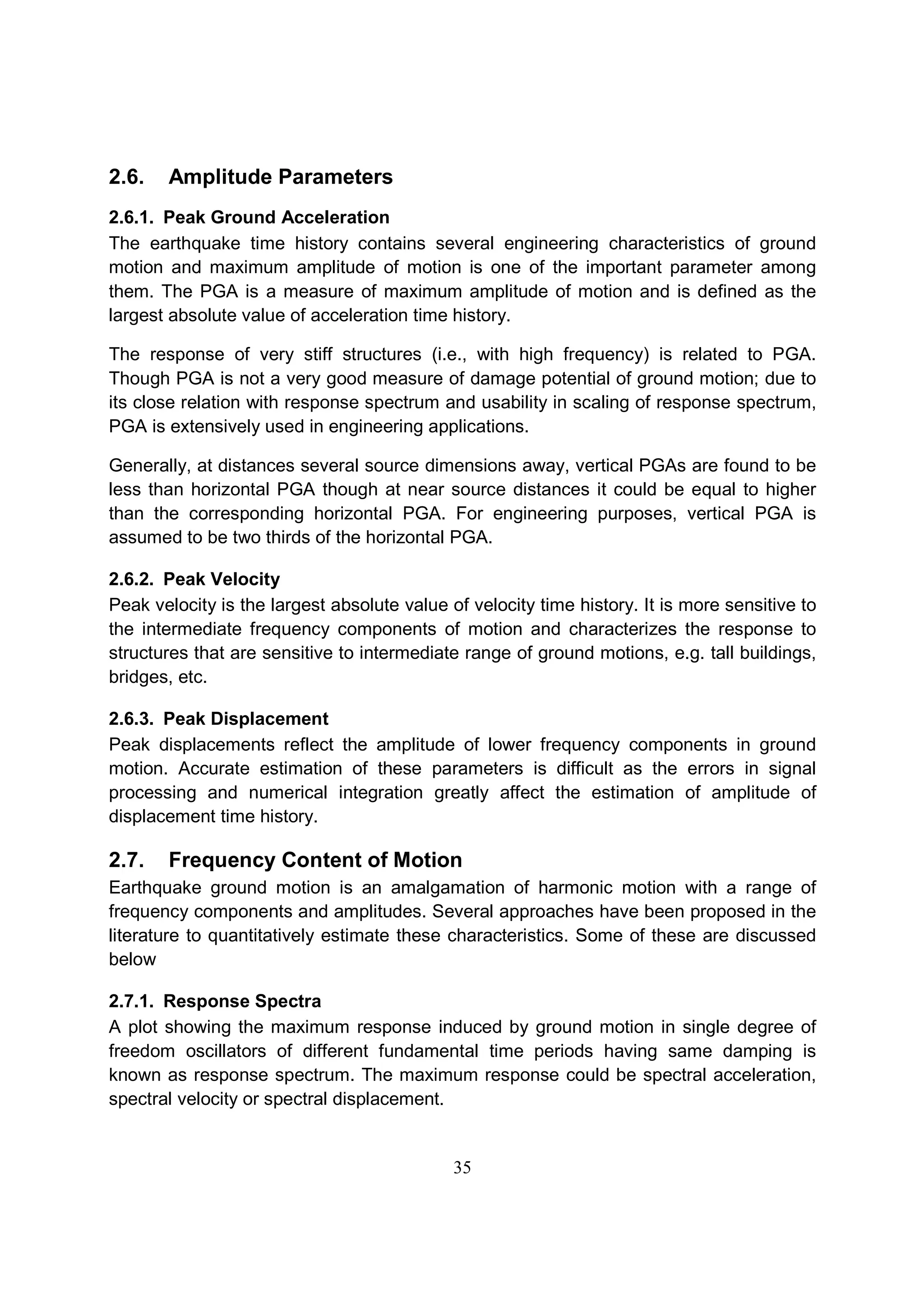
Figure 2.16 Mean + 1 sigma spectra predicted by Campbell & Bozorgnia (2008),
Atkinson & Boore (2006), Chiou & Youngs (2008) and Idriss (2008)
corresponding to a M6.0 earthquake at 20km distance and 15km focal
depth.
The recent attenuation relations also report the coefficients from which not only PGA but
also the spectral ordinates can also be derived. Using this approach, a complete
response spectrum can be derived directly from attenuation relations. Figure 2.16
depicts the mean + 1 sigma spectra obtained using the attenuation relationships
available in the literature
For some sites the design spectrum could be the envelope of two or more different
spectra. Such sites are affected by more than one active fault. The design spectra
obtained by considering the earthquake occurring from the two faults are different,
Figure 2.17.
Figure 2.17: Estimation of design response spectrum from multiple scenarios (From
Datta, 2010].
0
0.1
0.2
0.3
0.4
0.5
0.6
0.7
0.1 1 10 100
Frequency, Hz
SA,'g'
Campbell - Bozorgnia, 2008, Vs = 760
Atkinson - Boore (2006) ENA hard rock
Chiou and Youngs (2008), Vs1500
Idriss, 2008, Vs=900](https://image.slidesharecdn.com/02chapter-160115132216/75/02-chapter-Earthquake-Strong-Motion-and-Estimation-of-Seismic-Hazard-21-2048.jpg)
![51
2.11.2. Probabilistic Seismic Hazard Analysis [AERB, 2008; Roshan and Basu,
2010]
Determination of ground motion parameters by probabilistic method is accomplished by
performing a probabilistic seismic hazard analysis (PSHA). The subject of PSHA of a
site was initiated by Cornell (1968). Unlike maximisation of single valued earthquake
events as in deterministic approach, probabilistic approach takes into account the
probable distribution of earthquake magnitudes in each source, probable distances
within that source where earthquakes could originate and dispersion of acceleration
estimated using attenuation equations. In PSHA methodology, occurrence of
earthquakes is usually considered as Poisson process. This means that the events
have an average occurrence rate and could occur independent of the time elapsed
since last event.
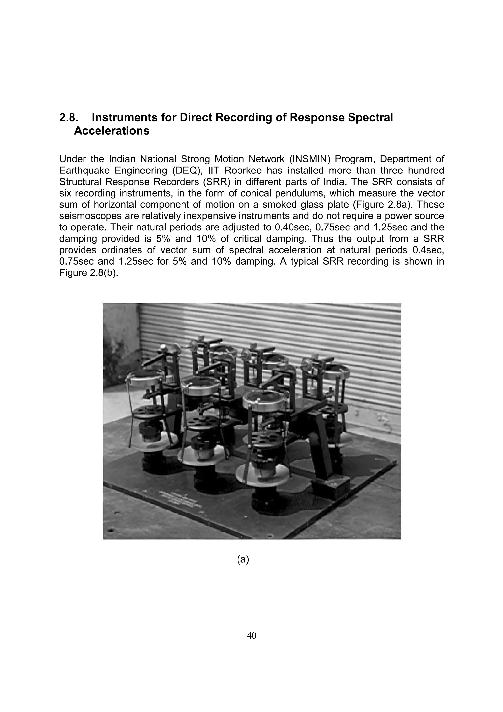
PSHA involves four steps (Figure 2.18):
• Specification of the seismic-hazard source model(s) (zonation);
• Specification of earthquake recurrence relationships which reflect earthquake activity
in the source
• Specification of the ground motion model(s) (attenuation relationship(s)); and
• The probabilistic calculation.
The seismic hazard is determined from the following form of expression:
∫ ∫∑
∞=
==
>=>
im
m
r
r
ii
N
i
i drdmrmzZPrfmfzZE
max,
min 01
),()()()( α (2.14)
Left side of equation (2.14), E(Z>z), is the frequency that acceleration Z being greater
than z. For obtaining the probability, one has to consider the temporal distribution of the
earthquake, which is normally taken as a Poisson process.
For PSHA of a site, earthquake sources within a defined region containing the site are
considered. These sources, depending on its characteristics are modeled as point, or
line, or aerial, or volume sources. Each source is assigned a maximum potential
magnitude mmax,i of earthquake. Total number of such sources (N) to be considered in
the PSHA study, their geometry and value of mmax,i are derived from the geological and
seismological information of the region/area around the site, and past earthquake data.
One value of minimum earthquake magnitude, mmin is generally assigned to all sources
from practical consideration of hazardous effect of minimum earthquake that can affect
the facility under consideration.
Activity rate of each source, αi, is determined from the earthquake recurrence
relationship of the region/source/fault based on Gutenberg-Richter relationship,
( ) bmamn −=10log (2.15)
Where n(m) is the number of earthquakes with magnitude m or greater per unit time,
and ‘a’ and ‘b’ are constants representing the seismic activity of the region/source/fault.](https://image.slidesharecdn.com/02chapter-160115132216/75/02-chapter-Earthquake-Strong-Motion-and-Estimation-of-Seismic-Hazard-22-2048.jpg)
![52
The alternate form of Guttenberg-Richter relationship is,
( ) m
0n m e−β
= ν (2.16)
In which, a
100 =ν and 10lnb=β .
The activity rate is the rate of earthquake corresponding to mmin and is given by,
min
0
m
e β
να −
= (2.17)
αi is calculated from α
The probability distribution of earthquake magnitude fi(m), is related to β, mmin and mmax,i
and generally follows the probability distribution function:
( )
( )[ ]
( )[ ]
[ ]minmax,
min
1
mm
mm
i i
e
e
mf −−
−−
−
= β
β
β
(2.18)
For estimation of α as well as )(mfi , the recurrence relation for the sources, i.e., ‘a’ and
‘b’ values needs to be determined from the earthquake database of the region under
consideration.
Figure 2.18: Various steps associated with probabilistic seismic hazard analysis.
(a) Zonation of earthquake sources
Line
Source
Mmax=6 Aerial source1
Mmax=6.5
Aerial source2
Mmax=7
SITE
Upper Bound cutoff
for magnitude, = Mmax
(b Reccurrence
(c) Attenuation
10% in 50 years (Return period = 475 years)
2% in 50 years (Return period = 2500 years)
(d) Hazard computation
Shaded area = P(Z>z|m,r)](https://image.slidesharecdn.com/02chapter-160115132216/75/02-chapter-Earthquake-Strong-Motion-and-Estimation-of-Seismic-Hazard-23-2048.jpg)


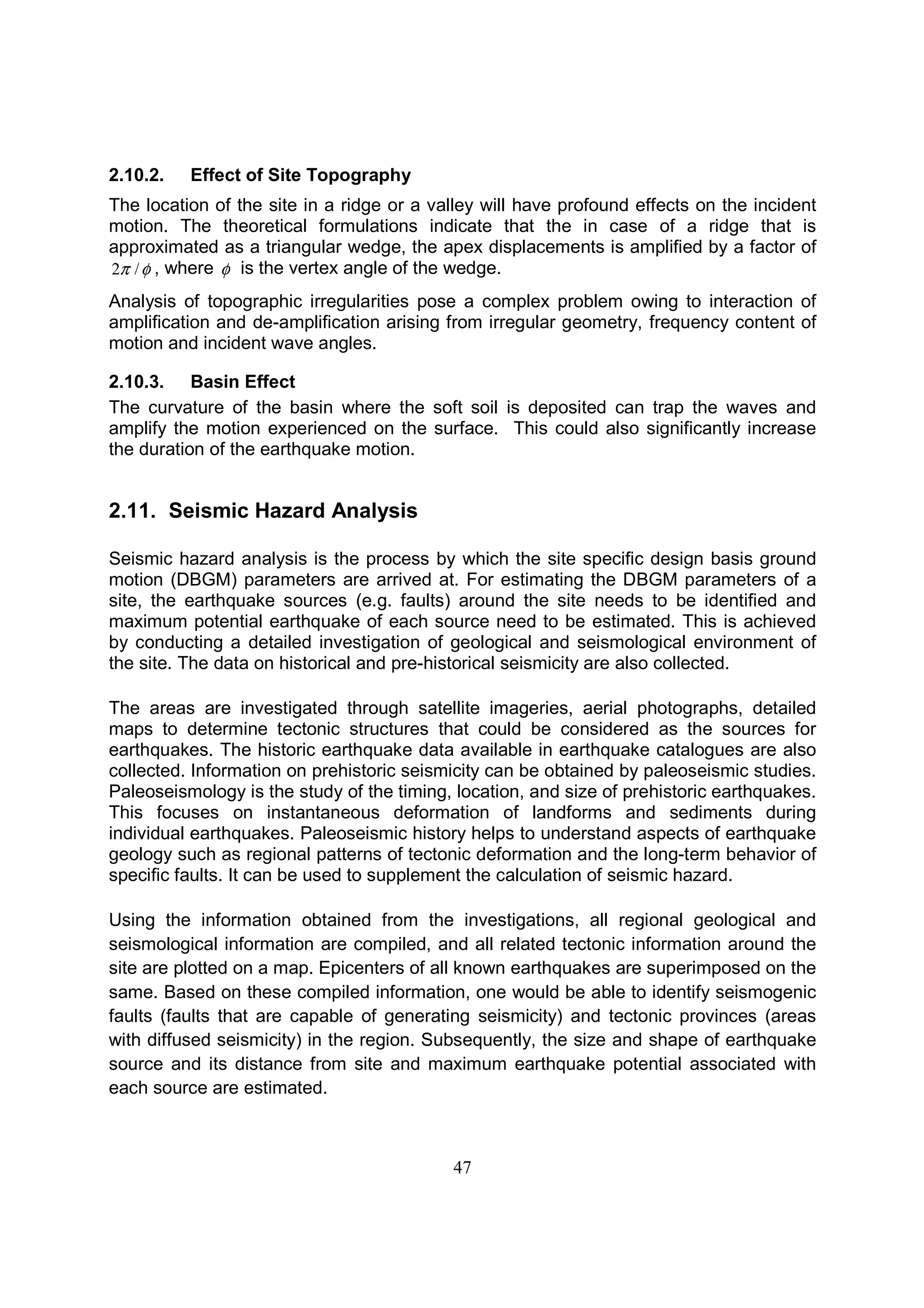
This document discusses strong ground motion from earthquakes and methods for measuring and analyzing it. It describes how modern accelerographs can record ground acceleration digitally up to 100 Hz. Parameters derived from ground motion records are used to analyze earthquake and site characteristics and their impact on structures. Evaluating seismic hazard requires understanding characteristics controlling ground motion as well as the seismicity and tectonics of the surrounding region, using either deterministic or probabilistic approaches.