The theory of error presentation

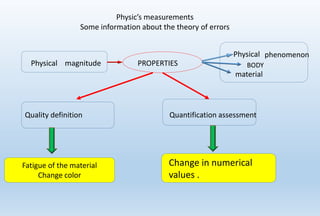
1. Quality definition Quantification assessment
phenomenon
material
Fatigue of the material
Change color
Change in numerical
values .
Physic’s measurements
Some information about the theory of errors
Physical magnitude PROPERTIES
Physical
BODY

2. Physical magnitudes and units of measure
Classification
a) Scalar [ numerical value ]
b) Vector- v , F , E
TIME -t
- weight mass -m , volume - V
ELECTRICAL CHARGE- e
c) Tensor Determine - the properties of the substance.
Physical magnitude units of measure
-Electrical permeability-
-Magnetic permeability H/m , N/A2
-Conductivity- G 1S = 1 Ω
Coefficient of thermal conductivity w/(m.K)
mF /


3. The system-SI
Magnitude Description UNIT DIMENSION
1. LENGTH L L=[m], meter dim L= L
2. WEIGHT M M=[m]=kg,
kilogram
dim m =M
3. TIME t [t]=s, second dim t = T
4. ELECTRIC CURRENT I [I] = A, amperes dim I=I
5. THERMODYNAMIC
TEMPERATURE
T [T] = K, Calvin dim T =θ
6. QUANTITY
SUBSTANCE
n [n] = mol, dim n = N
7. INTENSITY OF LIGHT J [J] = cd, candela dim J = J
Basic physical magnitude

4. Additional units
Physical magnitude Unit dimension
Flat angle rad
Spatial angle srad
r
s

2
r
A

8,4417571 ''0
rad
2
/1 rA

5. Dimensionless physical magnitude
friction coefficient NF /
Reynolds number
;
.
;
..




L
R
L
R
S
e
S
e



6. Type of measurements
1. Measuring directions-Direct comparison of a physical
magnitude with its unit of measure.
A = { A} [ A] , m = 0,20 kg is 5 times less than 1 kg
Example-L,m,t
2.Indirect measurements.

 JNITMLAdim
V
m


7. Indirect measurements -power consumption
sec1
1
1
J
W
IUP
t
W
P
IUtqUW
q
W
U





8. Information about the theory of errors
Lambert
The Foundations of Error Theory was established by Lambert in
1660-1765. Investigates measurement errors and classifies them.
The errors are:
1) Gross errors –Large diversion from the the real value of the measured
magnitude.
True value 23.7 Reported value - 37.2
2)Systematic errors
2.1 Instrumental errors -Limited accuracy of measuring equipment.
2.2 Subjective errors- Neglect of some external factors.
2.3 Systematic errors –caused by the chosen method of measurements
3.Random errors –If the measurements are made many times ,the results
are diferent
The reported values are larger or smaller than the true values
U(true)-(20-дел) =20v ,U(report)(20-дел)=2,5V

9. Random mistakes–Changing experience conditions .Incorrect
calculations, not an accurate measurement.
1. Measurement of current -I[A] through a resistor with resistance R.
The voltage U is measured on the resistor
with a voltmeter. Ohm's law is applied, there
is no internal resistance.
][
][
][


R
VU
AI Gross errors
Correct determination-Every voltmeter has an internal resistance-
RV.
U
RR
RR
I
V
V
 Correct calculation

10. 4.Systematic errors in indirect measurements
g
l
T 2 l
T
g 2
2
4

 sin
2
42
2
2
....
2
sin
64
9
sin
4
14










T
l
IF the angle is not small0
Then, a correction is added.

11. 5.ABSOLUT ERRORS
X Measured value
0X True value obtained with a reference device.
XXX  0
XniXXX i  ,).....3,2,1(0
mXmXmX 005,0,805,1,800,10 
mXmXmX i 105,0,650,320,755,3200 

12. 3. Relative errors
 X 0X
 
....000327,0
320755,0
000105,0
755,320
105,0
5,32075
5,10
320755
105
...,00277,0
00180,0
000005,0
180
5,0
1800
5
)(0
0






km
km
m
m
см
см
mm
mm
X
X
km
km
сm
сm
mm
mm
X
X
et
et
touereiffel
Ч
men


Note It does not depend on the choice of unit of measure. . Provides the
ability to compare precision measurement of magnitudes of different
dimensions : The period of rotation of the moon around the Earth and the
average radius of its orbit.

The ratio of absolute error to the true value of the phys. value-

13. 3. Relative error
The choice of relative error is due to the fact that:
1. The choice of unit of measure for the absolute error may be very small, but
its relative part of the value of the measured value can be significant.
mmmmkmX MEN 50005005,0000005,0)( 

14. Example of a relative error
Technical balance with precision gX 1,0
%025,0100.
400
1,0
%100.
%25,0100.
40
1,0
%100.
0
2
0
1










gX
X
gX
X


Technical balance with precision gX 0001,0
%000025,0100.
400
0001,0
%100.
0





gX
X


15. Accuracy class
V
X
X
k 5,2%100.
max



V
Xk
X 5,12
100
500.5,2
%100
. max


16. Presentation of experimental results
VU 60max  5,2k
VUизм 74,43
V
VkU
U 5,1
100
5,2.60
100
.max

   VUUU измREZ 5,174,43.. 
 VUREZ 5,17,43 
7,4374,43 

17. Make round of the results from the calculations.
13,0133,01326,0)1 
Example:
  %2,2%100.133/3 
Rounding rule
 
 
 
274.12735.1)2.3
274.12745.1)1.3
5)3
;273.12734.15)2
;274.12738.15)1





a
a
a
-The previous number does not change if it is even
-Increase by one the previous figure if it is odd

18. Statistical experimental results
The true value of –X0 is often unknown .Formula from the theory of
errors,which we will use .When the measurements are n .
1.(X1 ,X2 , X3 , ….,Xn )–are values of the researching magnitudes.
1.Mean value will be :)(X




n
i
i
n
X
nn
XXX
X
1
21 1............
)(X Is the closest to the real ones if n
nn XXX
XXX
XXX



....................
; 22
112.Deviation
The each separate deviation of the
measurements can be (+) or (-) .

19. Quantitative estimation of the arithmetic mean most
probable value for a finite number of measurements
3.Root means squared errors i.e .standard deviations –(SD)
 
 
)1.(
2
1




nn
XX
X
n
i
i
   )(3 XXX i  -Gross error
The results are represented by the average arithemetic value from the
particular finite number measurements X
 XX REZ

20. Random errors
p
XX
Когато n ∞   021 .....
1
XXXX
n
n 
 
 
1
2
1




n
XX
X
n
i
i

The common distribution law of the random errors is normal
distribution .This law is shown with Gaussian curve
Mean square deviation of a random
magnitude for a Xi measurement.
If the result is represented like :



3
2



XX
XX
XX
Possibility is:
%99
%95
%68



P
P
P

21. CONFIDENCE INTERVAL-d
n
t
Xd
np,
    XXXXtXtX npnp  ;.;. ,, 
npt ,
npt , Coefficient of Student . P-The probability ,that this interval contains the
true value ,n-number of measurements.
Coefficient of Student
n/P 50% 60% 70% 80% 90% 95% 99,9%
1 1,000 1,376 1,963 3.078 6,314 12,71 636,6
2 0,816 1,061 1,386 1,886 2,920 4,303 31,60
3 0,765 0,978 1,250 1,638 2,353 3,182 12,92
4 0,741 0,941 1,190 1,533 2,132 2,776 8,610

22. Indirect measurement errors
 00 )()()1( XfXXfXf  ERRORS OF COMPLEX MAGNITUDE
XXfXf  ).()()2(
Example:
ma 250,0
ma 001,0
 
3
3223
3333
)00019,001562,0(
0001875,0001,0.250,0.3.
;015625,0250,0
mV
mmmaaV
mmaV
REZ 




)()()1( aVaaVV 
   33333
00019,000018825,0250,0001,0250,0 mmmV 

23. Indirect measurement errors
KJCONSTX
XfXfXffXXX
J
nnn


,
...........;......, 221121
cma )1,00,21( 
 cmb 1,03,15 
 cmc 1,06,7 
33
88,24416,7.3,15.21.. cmcmcbaV 
     
;60718,59.....
;.........
33
cmcmcbabcaacbV
ccbabcbaacbaV cccccc








Error Rounding - Contains only the first significant
digit
1 cba
    3131
10.624410.688,2441 cmcmVREZ 

24. Indirect measurement errors
mmR )1,03,7(  01,0,14,3  
2
2222
222
2222
)2,13.167(
2,1161,1)1,0.14,3.201,0.3,7(
;..2...1.).(..
;331.1673,7.14,3.
cmS
cmcmcmS
RRRRRRS
cmcmRS
REZ 






25. Determining the error of a value expressed by
multiplication and grading
;)2(4)1(4)2(4
)(4)(4)(.4,...4
..4
32222
22222222
2
2
TTLLTLTg
TTLLLTLTgTL
T
L
g







It is divided the two sides of the error of g
.....,..........
......................
22
,)2(2
,
2
4424
4
3
3
2
2
1
1
321
3
2222
1
2
2
X
X
X
X
X
X
f
f
XXXf
T
T
L
L
g
g
T
T
L
L
g
g
T
T
LLTLT
T
L
g
g









































 










26. Least squares method
Yi Xi
Y1 X1
Y2 X2
…… ……
Yn Xn
Табл.1  
      
   
  
2
,
)(
.
,,,,
0,0,,)(
,)(
2
1
2
2
11
2
22
1 1
22
1
2
2
1
2
21
22
111
2
1
2
1




















 





 




N
bXaY
XXN
N
XXN
X
bandаforError
n
X
X
n
YX
XYXaYb
XX
YXXY
a
solutions
baXYSbXaXYXSYbaXSYbaXXP
YXPS
n
i
ii
Y
Y
n
i
i
n
i
i
aYn
i
n
i
ii
n
i
i
а
n
i
i
n
i
ii
n
i
iib
n
i
iiiia
n
i
ii
n
i
iiK



27. Simple linear regression
Y X
Y1 X1
.... ……
Yn Xn
Табл.2 XY 10  
 
 
  


 

















n
i
n
i
i
n
i
iiY
n
i
iX
n
i
iiXYXXY
YXXY
n
i
ii
X
n
XY
n
YYY
n
SXY
XX
n
SYYXX
n
SSS
RSSSR
SS
XYS
1 11
22
10
1
22
1
2
1
10
2
1
10
;
1
,
1
;
1
1
;
;
1
1
;))((
1
1
;/
11);(/;0;0;





28. 0,300 30,0
0,275 22,47
0,287 28,6
]/[ mmdBL   ][ mDx Al 
1.0
1.0
1.0
y = 0,0029x + 0,2087
R² = 0,8686
0.26
0.27
0.28
0.29
0.3
0.31
0 10 20 30 40
We can show the results of the measurements as table, as
graphic or analytically
]/[ mmdBy L
][ mDx Al 
bDmL  .

29. Summary
1) The independent measurements (n ) are made of the magnitude X
2)We write the results X1 ,X2,…….Xn in table.
3)We find the mean value .
4)The absolute errors has to be defined for each measurements
5) We define the standard deviation using the term .
6)The results
7) The absolute error e given with
X
),...,2,1( niXXX ii 
)1()1(
1
2
2
1






 
nn
X
nn
XX
n
i
i
n
i
i

nptXX ,.
,%
,
X
t
X
np 
