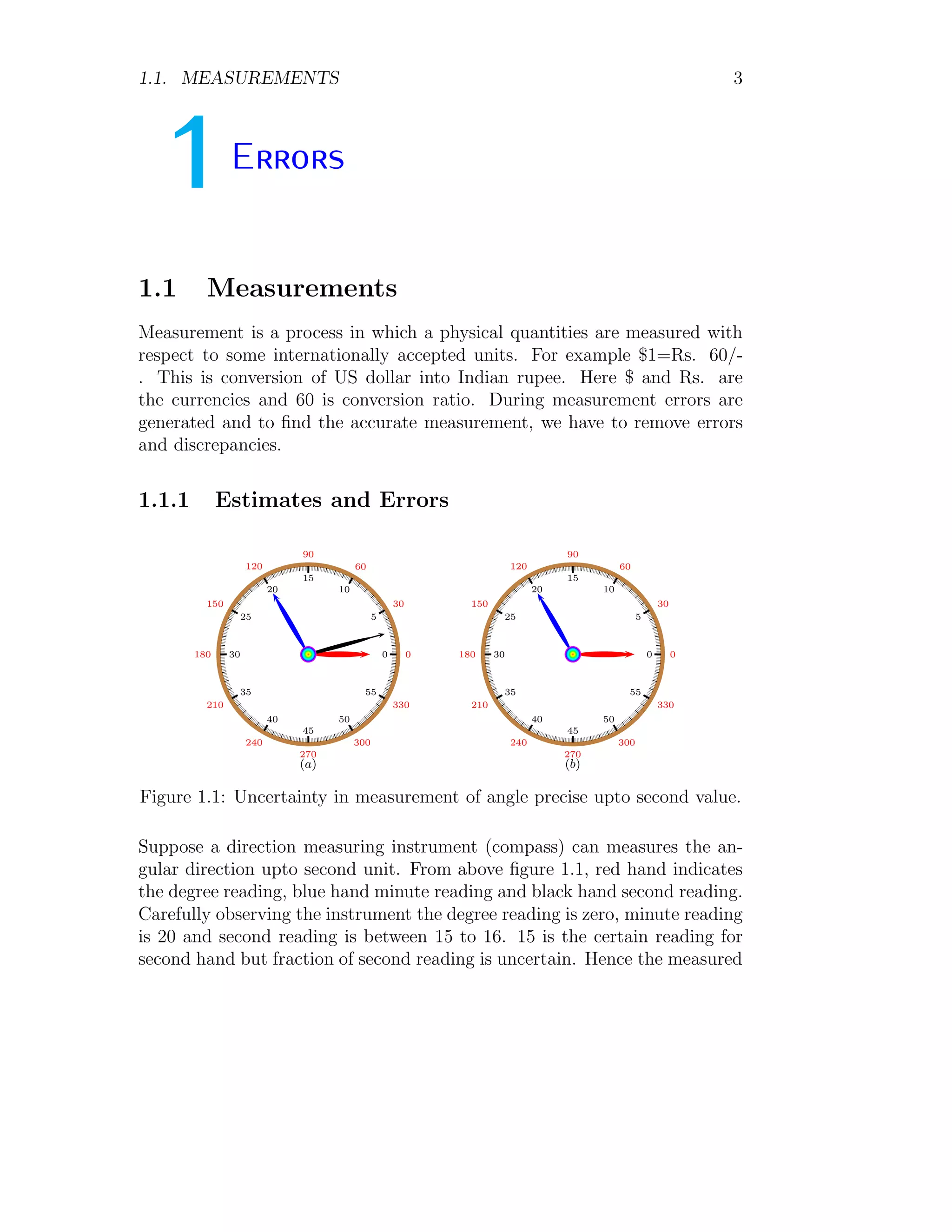
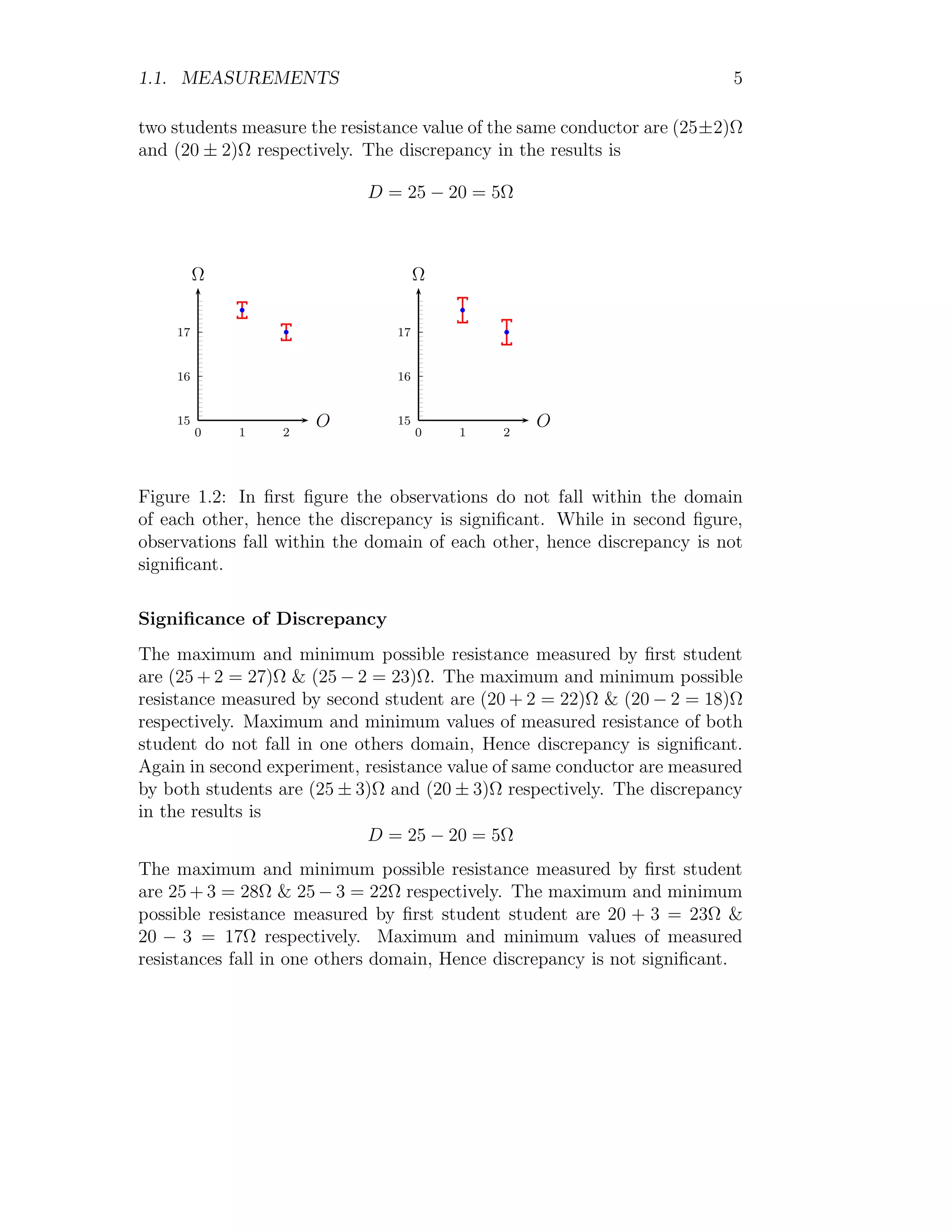
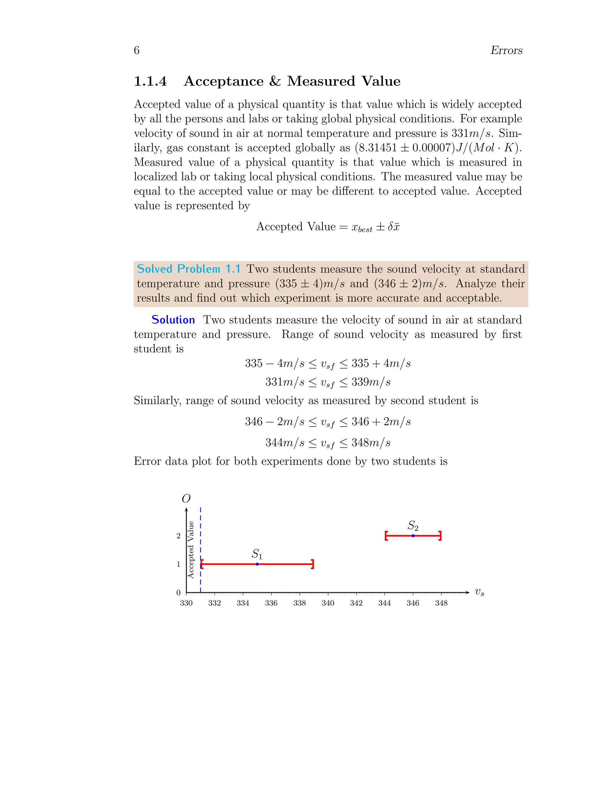
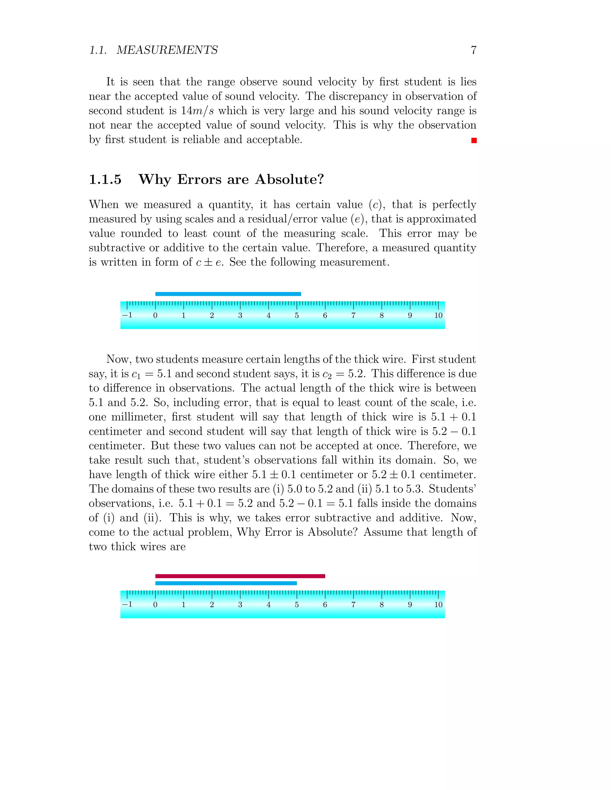
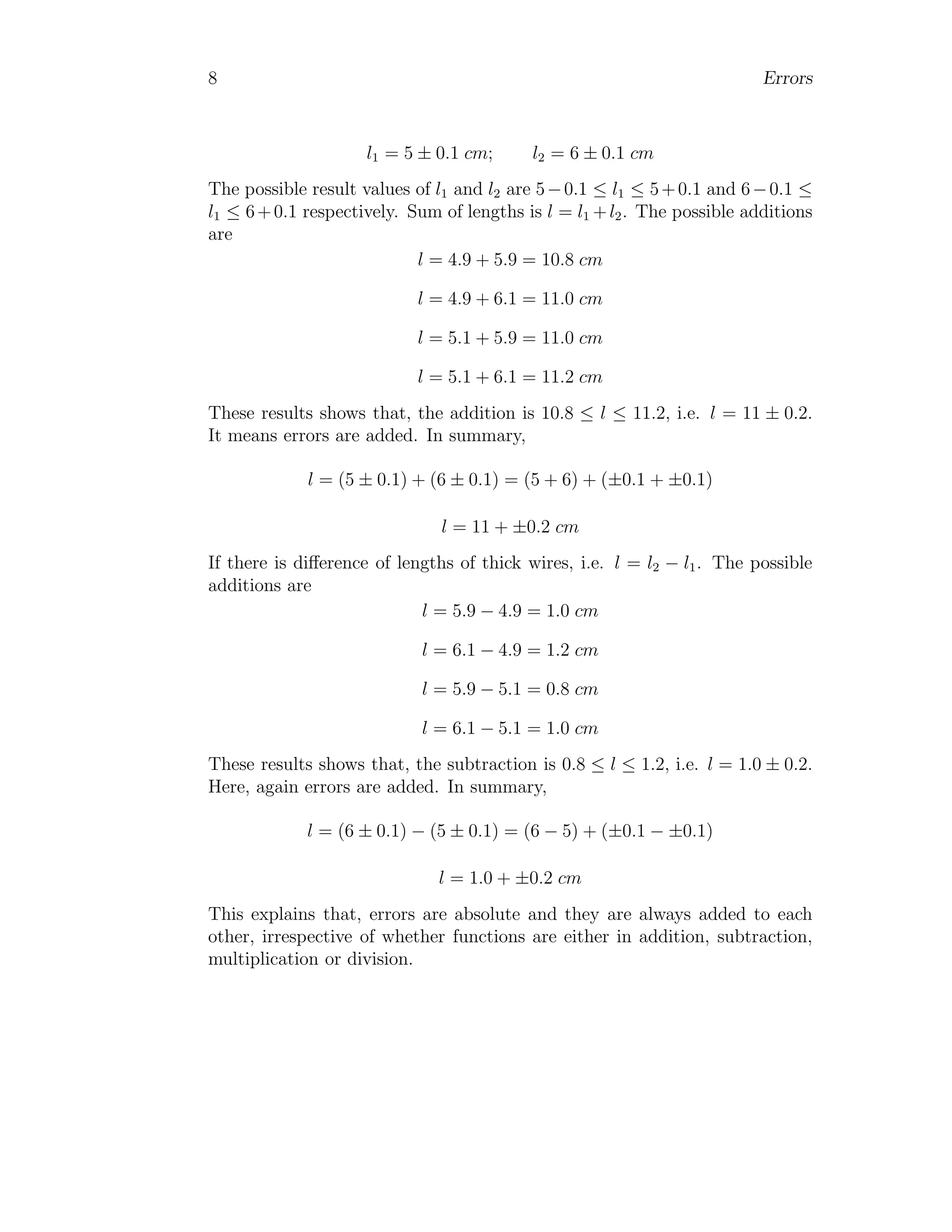
This note is calculus based error measurement. It explains how calculus can be used to find errors in functions and measurements. Best for quick revision before CBSE Board Examination.
This document defines key terms related to instruments and measurement:
- Accuracy refers to how close a measurement is to the true value. It is limited by the instrument's least count.
- Calibration establishes the relationship between instrument readings and measured quantities by comparing to standard instruments.
- Sensitivity is the ratio of change in the instrument reading to the change in the measured quantity. It quantifies how responsive the instrument is.
- Threshold refers to the minimum quantity needed for the instrument to provide a detectable reading.
This document is a lecture note from Ambo University's Department of Mathematics for an Applied Mathematics I course. It covers various topics in applied mathematics over 5 chapters, including: vectors and vector spaces, matrices and determinants, limits and continuity, derivatives and their applications, and integration. The document provides definitions, theorems, and methods for each of these fundamental areas of applied mathematics.
Measurement of Geometrical Errors in Manufacturing FlatnessSamet Baykul
DATE: 2018.11
This is an experiment report which is prepared for ME410 class in METU mechanical engineering department.
In this report, we will measure the straightness of line segments at certain intervals and calculate the flatness of a surface through these measurements. We will discuss how this measurement works. We will also discuss the results and possible errors.
Principle of Integration - Basic Introduction - by Arun Umraossuserd6b1fd
Notes for integral calculus. Students must read function analysis before going through this book. Read Derivative Calculus before going through this book.
Beginner's idea to Computer Aided Engineering - ANSYSDibyajyoti Laha
This document contains a student assignment containing various exercises involving calculations of stress and deformation of mechanical parts using analytical calculations and finite element analysis (FEA) in ANSYS. The exercises involve cylindrical bars, cantilever beams, hollow beams, and combined struts under various loads. The student provides the part dimensions, applied loads, material properties, screenshots of the FEA models, and compares the results of calculations to FEA results, noting good agreement overall with some differences explained by modeling approximations.
1. The document provides an introduction to physics concepts including understanding physics, base and derived quantities, scalar and vector quantities, and measurements.
2. Key concepts discussed include the definition of physics, base units, derived units, scalar and vector quantities, and factors that affect the accuracy and sensitivity of measuring instruments.
3. Examples are provided to illustrate scientific notation, unit conversion, identifying systematic and random errors, and the proper use of instruments like the vernier caliper and micrometer screw gauge.
This document discusses the analysis of a cantilevered L4x4 aluminum beam. It includes:
1. Computing section properties like centroid, moments of inertia, and flexibility matrix of the beam. Values from SolidWorks were compared.
2. Calculating stresses from bending, shear, and torsion at various points on the cross section.
3. Determining displacements and rotations of the beam tip under an applied load using the flexibility matrix in MATLAB and comparing to an Abaqus model. Percentage errors between analysis methods were reported.
Reliability Analysis of the Sectional Beams Due To Distribution of Shearing S...researchinventy
This paper shows the results of the Reliability Analysis of the sectional beams due to distribution of Shear Stress. It is assumed that the load was uniformly distributed over the beam. It is discussed that the distribution of shear stress over the beam. It is discussed that the average shears stress and maximum shear stress across the section of the beam for Weibull distribution. The reliability analysis of distribution of shearing stresses over sectional beams is performed. Also it is derived that the hazard functions for these types of beams. Reliability comparison has also been done for the sectional beams. It is observed that the reliability of the beam decreased when the width (b) of the beam decreases, and the load (F) is high. The reliability of the beam is increased when the height (h) of the triangular section increases , diameter(d) of the circular beam is increased and parameter 푘 decreasses
1. The document discusses physical magnitudes and units of measurement. It defines scalar and vector physical magnitudes like time, mass, volume, and electrical charge.
2. The International System of Units (SI) is presented, which standardizes seven base physical quantities like length, mass, time, electric current, temperature, amount of substance, and luminous intensity.
3. Types of measurements are described including direct comparison and indirect measurements. Methods for determining errors in direct and indirect measurements are also covered.
1. This document provides guidance for answering physics questions on a practical exam involving experiments.
2. Section A involves 2 structured questions based on experiments students should have performed. Questions will require identifying variables, recording data in tables, plotting graphs, and determining relationships from graphs.
3. Section B involves answering one question describing an experimental framework to test a hypothesis related to a diagram and situation described. The description must include the aim, variables, apparatus, procedure, data collection method, and data analysis.
Stress Analysis of Chain Links in Different Operating Conditionsinventionjournals
The work covers the stress analysis in a 3D model of chain link analitically and numerically, and based on a real model, experimental examination was carried out. First, the cases when the links are vertical to each other and their tensile load were considered. The analysis was done in both work and experimental conditions and also the tensile load just before the chain broke. Second, the position in which the links are rotated for the calculated maximum angle. Experimental analysis of the high resistance chain (high hardness), insignia stress 14x50 G80 E5 was carried out on an universal testing mashine and the results are used for verification of numerical model.
Development of a test statistic for testing equality of two means under unequ...Alexander Decker
This document proposes a new test statistic for testing the equality of two means from independent samples with unequal variances (known as the Behrens-Fisher problem). It develops a test that uses the harmonic mean of the sample variances instead of the pooled variance. Through simulation, it determines the degrees of freedom for the distribution of the harmonic mean that allows it to be approximated by the chi-square distribution. It then provides an example application to agricultural yield data to demonstrate how the new test statistic can be used.
The document discusses statistical techniques used to analyze data through frequency distributions and measures of central tendency. It provides information on how raw data is organized into class intervals and represented graphically using histograms, frequency polygons, and calculations of mean, median, and mode. Standard deviation is introduced as a measure of how concentrated data are around the mean. Examples are given on calculating mean, variance, and standard deviation for both raw data and grouped frequency distributions. The normal distribution is also described along with how it can be used to calculate probabilities based on areas under the standard normal curve.
The document defines variance as the average of the squared differences from the mean. It provides examples of calculating variance and standard deviation for different data sets involving heights of dogs, exam scores, and word counts per page. Variance is found by taking the difference of each value from the mean, squaring it, and averaging the results. Standard deviation is the square root of the variance.
The document discusses vectors and vector arithmetic. It defines scalars and vectors, and explains that vectors have both magnitude and direction while scalars only have magnitude. It then discusses how vectors can be represented geometrically using arrows and how any two-dimensional vector can be decomposed into two components. The bulk of the document focuses on vector arithmetic, describing how vectors can be added and multiplied through various methods like the parallelogram law of addition, triangle law of addition, and scalar multiplication. It provides examples of how these vector arithmetic operations can be used to model real-world phenomena like displacements caused by earthquakes.
This document provides tips for taking online classes, including being prepared before class, treating it like a real course, managing time well, creating a dedicated study space, eliminating distractions, participating actively, and leveraging your network. It also outlines expectations for participating in online classes, such as keeping your camera on, muting your audio, taking notes on your own materials rather than on the shared screen, and only speaking or sharing after getting permission.
Please Subscribe to this Channel for more solutions and lectures
http://www.youtube.com/onlineteaching
Chapter 6: Normal Probability Distribution
6.6: Normal as Approximation to Binomial
This document discusses concepts related to error analysis and statistics. It covers accuracy and precision, individual measurement uncertainty including means, variance, standard deviation and confidence intervals. It also discusses uncertainty when calculating quantities from multiple measurements using error propagation. Additionally, it discusses least squares fitting of data. Key points include how to quantify accuracy and precision, characterize the distribution of data, calculate uncertainty intervals, and propagate errors through calculations involving multiple measured variables.
This lab report investigates the relationship between the number of spaghetti strands and the applied force needed to break them. The experiment involved placing different numbers of spaghetti strands (2, 3, 4, 5, 6) on a platform and measuring the force required to break them using a dynamometer. The results showed that as the number of spaghetti strands increased, the average applied breaking force also increased. A direct proportional relationship between the number of spaghetti strands and applied force was determined. The hypothesis that increasing the number of spaghetti strands would increase the breaking force was supported.
This lab report investigates the relationship between the distance and time it takes for dominoes to fall in a chain reaction. The experiment measured the falling time of 10 dominoes placed at distances of 1-5 cm. The results showed that as the distance between dominoes increased, the average falling time also increased from 0.82 seconds at 1 cm to 1.35 seconds at 5 cm. A graph of these results displayed a direct proportional relationship between distance and time. The report concludes that the hypothesis that increasing distance leads to increasing falling time was supported. It suggests improvements such as using a pendulum to apply a more consistent initial force to the dominoes.
Hertz Contact Stress Analysis and Validation Using Finite Element AnalysisPrabhakar Purushothaman
In general machines are designed with a set of elements to reduce cost, ease of assembly and manufacturability
etc. One also needs to address stress issues at the contact regions between any two elements, stress is induced when a load is applied to two elastic solids in contact. If not considered and addressed adequately serious flaws can occur within the mechanical design and the end product may fail to qualify. Stresses formed by the contact of two radii can cause extremely high stresses, the application and evaluation of Hertzian contact stress equations can estimate maximum stresses produced
and ways to mitigate can be sought. Hertz developed a theory to calculate the contact area and pressure between the two
surfaces and predict the resulting compression and stress induced in the objects. The roller bearing assembly and spur gear pair assembly is an example were the assembly undergoes fatigue failure due to contact stresses. This paper discusses the hertz contact theory validation using finite element Analysis.
The document provides information about a physics textbook published by DISHA PUBLICATION. It states that no part of the publication may be reproduced without permission from the publisher. It provides contact information for DISHA PUBLICATION, including their address in New Delhi, India, email, and websites. It also includes a table of contents for the textbook that lists 28 chapters and their corresponding page numbers and question numbers.
To calculate the thermal expansion coefficients (α1 and α2) for a lamina with a fiber and matrix, the following steps are taken:
1. The total strain is calculated as the sum of the mechanical and thermal strains.
2. Equations are developed relating stress, strain, and thermal expansion for directions 1 and 2.
3. The equations are set equal to determine expressions for α1 and α2 in terms of the fiber and matrix thermal expansion coefficients and volume fractions.
4. The final expressions obtained are α1 = (αfEfVf + αmEmVm)/E and α2 = αmVm + αfVf.
This document is a study guide for an introductory abstract algebra course. It was written by John A. Beachy of Northern Illinois University as a supplement to the textbook "Abstract Algebra" by Beachy and Blair. The study guide provides solved problems and explanations for key concepts in integers, functions, groups, polynomials, rings, and fields to help students learn the material. It is intended to help students who are beginning to learn abstract algebra and having to write their own proofs.
Diploma sem 2 applied science physics-unit 1-chap 2 error sRai University
This document discusses various types of errors that can occur in measurements. It describes instrumental error, observer error, and procedural error as the three main sources of uncertainty. It also defines accuracy as a measure of how close a measurement is to the accepted value, while precision refers to the closeness of repeated measurements. The document provides examples of calculating percentage error, relative error, and discusses significant figures when taking measurements.
R = R0(1 + α(t - 20))
- The resistance (R) of a copper wire is calculated using a formula that relates it to the resistance at 20°C (R0), the coefficient of resistance (α), and the temperature (t).
- R0 is given as 6Ω with an uncertainty of ±0.3%.
- To determine the uncertainty in R, the uncertainties in R0, α, and t must be determined and propagated through the equation using partial derivatives.
- The overall uncertainty in R combines the individual uncertainties from each variable according to the propagation of uncertainty formula.
This document outlines types of errors in measurement and uncertainty analysis. It discusses procedural, human, random, instrumental, environmental, and approximation errors. It also covers precision versus accuracy, resolution versus sensitivity, and the importance of estimating errors before and during experiments. Methods are provided for estimating errors in individual measurements using least counts, fluctuating displays, steady displays, extrapolating readings, and inability to judge readings clearly. The document stresses estimating uncertainties before experiments to determine needed measurement accuracy and significant figures in reported values.
This document covers several topics related to measurement and error analysis in physics experiments. It begins by defining accuracy and precision, distinguishing between the two concepts. Accuracy refers to how close a measurement is to the true value, while precision describes the degree of variation in repeated measurements of the same quantity. It then discusses random and systematic errors, explaining that random errors vary unpredictably while systematic errors remain constant. The document provides examples of different types of systematic errors like instrumental, environmental, and observational errors. Finally, it introduces concepts like absolute error, relative error, and percentage error to quantify the uncertainty in measurements.
This document discusses uncertainties and errors in physical measurements. It explains that there are two types of errors - random errors which are unpredictable, and systematic errors caused by imperfect measuring equipment. Random errors can be reduced by repeating measurements, while systematic errors are reduced by calibrating equipment. Accuracy refers to how close a measurement is to the true value, while precision refers to how close repeated measurements are. The number of significant figures reported in a result should not exceed the least precise value used. The document also discusses determining and expressing uncertainties in measurements, and how to combine uncertainties when performing calculations or graphing data.
1) The document discusses measurement and error in engineering. It covers characteristics of measuring instruments such as accuracy, precision, sensitivity, and error.
2) Accuracy refers to how close a measurement is to the true value, while precision refers to the reproducibility of measurements. Systematic errors can be corrected, while random errors average out over multiple trials.
3) Significant figures indicate the precision of a measurement. The number of significant figures retained in calculations is determined by the least precise measurement.
Introduction, types of errors, definitions, laws of accidental errors, laws of weights, theory of least squares, rules for giving weights and distribution of errors to the field observations, determination of the most probable values of quantities.
The document discusses experimental data and uncertainty. It explains that all data has some uncertainty due to limitations of instruments and humans. It also discusses accuracy, precision, and significant figures when reporting results. The mean, uncertainty in the mean, and fractional and percentage uncertainties are also covered.
Errors and Uncertainty are parts of surveying. These slides start first by defining scale and measurements, then show how to determine the uncertainty in measurements. For making these slides I used some books as well; Surveying_Engineering Surveying 6th edition, Surveying Problem Solving, & Surevying_Elemntary Surveying an introduction to Geomatics_Paul R. Wolf.
Dimensional analysis can be used to derive equations, check if equations are dimensionally correct, and find the dimensions or units of derived quantities. It involves identifying the fundamental dimensions - such as length, time, mass - of the variables in an equation. An equation is dimensionally correct if the dimensions on both sides are equal. For example, the equation for velocity, v=s/t, can be dimensionally checked as [v]=[s]/[t] which gives meters/second. Dimensional analysis allows deriving the formula for the period of a pendulum as T=2π√(l/g).
This document discusses the theory of errors in survey measurements. It begins with an introduction to the types of errors that can occur, including mistakes, systematic errors, and accidental errors. It then provides definitions for key terms like direct observation, indirect observation, conditioned quantity, true value, most probable value, true error, and residual error. The document goes on to explain statistical formulas used to calculate the probable error of single observations, the probable error of the mean, standard deviation, standard error, and precision. It also covers the law of accidental errors and laws of weights. Finally, it discusses the theory of least squares and provides examples of determining probable errors and finding the most probable value of quantities.
This document provides an overview of the theory of errors in survey measurements. It discusses the different types of errors including mistakes, systematic errors, and accidental errors. It defines key terms like true value, most probable value, true error, and residual error. Statistical formulas for probable error, standard deviation, and standard error are presented. Laws of accidental errors and weights that describe the distribution and weighting of errors are covered. The principle of least squares and its application in determining most probable values from observations is explained. Methods for calculating error in sums, error of the mean, and errors in indirect and conditional observations are also summarized.
1. The document discusses units of measurement and the SI system. It describes the seven base SI units including meters, kilograms, seconds, and kelvins.
2. Derived units are discussed along with examples like density. Significant figures and the accuracy and precision of measurements are also covered.
3. Errors in measurements are defined as the difference between experimental and accepted values. Percent error can quantify the accuracy of a measurement.
Measurement errors, Statistical Analysis, UncertaintyDr Naim R Kidwai
The Presentation covers Measurement Errors and types, Gross error, systematic error, absolute error and relative error, accuracy, precision, resolution and significant figures, Measurement error combination, basics of statistical analysis, uncertainty, Gaussian Curve, Meaning of Ranges
Physics is the study of the basic components of the universe and their interactions. Key aspects of the scientific method include making observations, developing theories to explain those observations, and making predictions with those theories that can then be verified or falsified by further observations. The International System of Units (SI) provides standardized base units for measuring various physical quantities. Proper measurement requires defining the physical quantity, choosing appropriate units, and accounting for the precision of the measurement.
This lecture discusses scientific measurements and units. It covers the metric system and SI units, dimensional analysis, unit conversions, and significant figures. Key points include:
1. The metric system uses meters, grams, and seconds as fundamental units. There are seven base SI units including the meter for length and gram for mass.
2. Dimensional analysis uses conversion factors to change between units while maintaining the correct dimensions. It is useful for solving chemistry problems.
3. Significant figures reflect the precision of a measurement and determine how many digits are reported in calculations. Rules for significant figures depend on the operation being used.
This lecture discusses scientific measurements and units. It covers the metric system and SI units, dimensional analysis, unit conversions, and significant figures. Key points include:
1. The metric system uses meters, grams, and seconds as fundamental units. There are seven base SI units including the meter for length and gram for mass.
2. Dimensional analysis uses conversion factors to change between units while maintaining the correct dimensions. It is useful for solving chemistry problems.
3. Significant figures indicate the precision of a measurement and how numbers should be rounded. Calculations are rounded according to whether they involve multiplication/division or addition/subtraction.
This document discusses measurement and uncertainties in physics. It introduces standard SI units which are used for measurement in most countries. Fundamental quantities like length, time and mass cannot be measured in simpler terms and form the basis of other derived units. Accuracy refers to how close a measurement is to the accepted value, while precision refers to the agreement between multiple measurements. Random and systematic errors can affect measurements and need to be accounted for using techniques like taking multiple readings and estimating uncertainties. Graphs are useful for analyzing experimental data and determining relationships between variables.
The document discusses a study that used LiF thermoluminescent dosimeters (TLDs) to perform in vivo dosimetry measurements on radiotherapy patients. Measurements of entrance dose, exit dose, and midline dose were taken and used to determine water-equivalent depth and target dose. Monte Carlo simulations were also conducted to examine interactions of gamma rays with LiF and the resulting electron spectra. The results showed close agreement between measured midline dose and expected values based on water-equivalent depth, and supported the use of a compact gamma ray spectrometer for in vivo dosimetry measurements up to energies of around 20 MeV.
Fisika Bilingual Besaran dan Satuan Kelas 7Frank Nanda
Ini adalah LKS (Lembar Kerja Siswa untuk Bab.Besaran dan Satuan di Kelas 7. Untuk memberi siswa wawasan lebih luas tentang kata-kata pada fisika yang ada di luar negeri.
Similar to Measurements of Errors - Physics - An introduction by Arun Umrao (20)
Notes for c programming for mca, bca, b. tech cse, ece and msc (cs) 1 of 5 by...ssuserd6b1fd
C programming language notes for beginners and Collage students. Written for beginners. Colored graphics. Function by Function explanation with complete examples. Well commented examples. Illustrations are made available for data dealing at memory level.
Decreasing increasing functions by arun umraossuserd6b1fd
1. The document defines functions and their domains and ranges. It discusses increasing and decreasing functions, where an increasing function's values continuously rise with x and a decreasing function's values continuously fall with x.
2. It provides an example of a function f(x) = x^2 - 5.5x + 6 that decreases from x = 1 to 2.7 and then increases from 2.7 to 4.5.
3. To determine if a function is increasing or decreasing over a domain, one calculates the first order differences between adjacent y-values and checks if the differences are positive or negative.
Distribution of normal data understanding it numerical way by arun umraossuserd6b1fd
The document discusses normal data distribution and provides examples. It defines normal data as being symmetrically distributed about the mean value, with 99.7% of data within 3 standard deviations of the mean. It then generates a sample of 50 random numbers between 14-18 and calculates the mean and standard deviation. A histogram of the deviations from the mean (x-μ) is plotted, showing the normal distribution curve shape.
Decreasing and increasing functions by arun umraossuserd6b1fd
Function analysis - characteristics of increasing and decreasing functions. How "sign" either positive or negative tells about the nature of the function, i.e. where it is increasing and where it is decreasing.
What is meaning of epsilon and delta in limits of a function by Arun Umraossuserd6b1fd
The document defines the limit of a function. It states that a function f(x) is defined on a bounded domain R and the limit is evaluated at a point x0 as x approaches x0 from the positive side. It defines ε and δ such that if |f(x) - f(x0)| < ε when 0 < |x - x0| < δ, then the limit of f(x) as x approaches x0 is f(x0). It provides an example of the limit of f(x) = 1/x as x approaches 0 and explains that the limit does not exist since ε is undefined.
Notes for GNU Octave - Numerical Programming - for Students 01 of 02 by Arun ...ssuserd6b1fd
The document provides an introduction to GNU Octave, an open-source software program for numerical computations. It covers various topics in mathematics, including expressions, arithmetic operators, comparison operators, evaluation, algebra, complex numbers, geometry, logarithms, and trigonometric functions. For each topic, it lists and briefly describes the relevant Octave commands and functions that can be used for computations and analysis.
Notes for C++ Programming / Object Oriented C++ Programming for MCA, BCA and ...ssuserd6b1fd
C++ programming language notes for beginners and Collage students. Written for beginners. Colored graphics. Function by Function explanation with complete examples. Well commented examples. Illustrations are made available for data dealing at memory level.
Think Like Scilab and Become a Numerical Programming Expert- Notes for Beginn...ssuserd6b1fd
Notes for Scilab Programming. This notes includes the mathematics used behind scilab numerical programming. Illustrated with suitable graphics and examples. Each function is explained well with complete example. Helpful to beginners. GUI programming is also explained.
Think Like Scilab and Become a Numerical Programming Expert- Notes for Beginn...ssuserd6b1fd
The document discusses Scilab, an open-source numerical computation software. It provides an introduction to Scilab's core functionality, including how it represents all data as matrices, performs simple arithmetic operations on matrices, and uses keywords to control program flow and perform other tasks. Some of the major keywords and functions covered are addition, subtraction, multiplication, division, square root, exponent, logical operators, for loops, if/else statements, and help functions like version and get memory.
Notes for C Programming for MCA, BCA, B. Tech CSE, ECE and MSC (CS) 5 of 5 by...ssuserd6b1fd
C programming language notes for beginners and Collage students. Written for beginners. Colored graphics. Function by Function explanation with complete examples. Well commented examples. Illustrations are made available for data dealing at memory level.
Notes for C Programming for MCA, BCA, B. Tech CSE, ECE and MSC (CS) 4 of 5 by...ssuserd6b1fd
C programming language notes for beginners and Collage students. Written for beginners. Colored graphics. Function by Function explanation with complete examples. Well commented examples. Illustrations are made available for data dealing at memory level.
Notes for C Programming for MCA, BCA, B. Tech CSE, ECE and MSC (CS) 3 of 5 b...ssuserd6b1fd
C programming language notes for beginners and Collage students. Written for beginners. Colored graphics. Function by Function explanation with complete examples. Well commented examples. Illustrations are made available for data dealing at memory level.
Notes for C Programming for MCA, BCA, B. Tech CSE, ECE and MSC (CS) 2 of 5 by...ssuserd6b1fd
C programming language notes for beginners and Collage students. Written for beginners. Colored graphics. Function by Function explanation with complete examples. Well commented examples. Illustrations are made available for data dealing at memory level.
Notes for C Programming for MCA, BCA, B. Tech CSE, ECE and MSC (CS) 1 of 5 by...ssuserd6b1fd
C programming language notes for beginners and Collage students. Written for beginners. Colored graphics. Function by Function explanation with complete examples. Well commented examples. Illustrations are made available for data dealing at memory level.
Notes and Description for Xcos Scilab Block Simulation with Suitable Examples...ssuserd6b1fd
This notes on xcos are similar to Simulink of Matlab. Suitable for easy block drawing and simulations for systems or mathematical problems. This notes also explains about the working of blocks, mathematics behind them - used for block computation - their structures and input-output data.
How energy relates to work? to know more, read this notes. Suitable for CBSE board students. Sections contains work energy, work energy units, work energy conversion
Physics dictionary for CBSE, ISCE, Class X Students by Arun Umraossuserd6b1fd
Dictionaries are very important. Without definitions of scientific words you can not understand the theories or theorems. This dictionary explains nearly all the terms used in CBSE Class X science book.
Java Programming Notes for Beginners by Arun Umraossuserd6b1fd
Shot notes for quick revision. Not explained extensively but suitable for last night preparation. Fit for CBSE Class XII board students for their last minute preparation.
Gender and Mental Health - Counselling and Family Therapy Applications and In...PsychoTech Services
A proprietary approach developed by bringing together the best of learning theories from Psychology, design principles from the world of visualization, and pedagogical methods from over a decade of training experience, that enables you to: Learn better, faster!
How to Setup Warehouse & Location in Odoo 17 InventoryCeline George
In this slide, we'll explore how to set up warehouses and locations in Odoo 17 Inventory. This will help us manage our stock effectively, track inventory levels, and streamline warehouse operations.
ISO/IEC 27001, ISO/IEC 42001, and GDPR: Best Practices for Implementation and...PECB
Denis is a dynamic and results-driven Chief Information Officer (CIO) with a distinguished career spanning information systems analysis and technical project management. With a proven track record of spearheading the design and delivery of cutting-edge Information Management solutions, he has consistently elevated business operations, streamlined reporting functions, and maximized process efficiency.
Certified as an ISO/IEC 27001: Information Security Management Systems (ISMS) Lead Implementer, Data Protection Officer, and Cyber Risks Analyst, Denis brings a heightened focus on data security, privacy, and cyber resilience to every endeavor.
His expertise extends across a diverse spectrum of reporting, database, and web development applications, underpinned by an exceptional grasp of data storage and virtualization technologies. His proficiency in application testing, database administration, and data cleansing ensures seamless execution of complex projects.
What sets Denis apart is his comprehensive understanding of Business and Systems Analysis technologies, honed through involvement in all phases of the Software Development Lifecycle (SDLC). From meticulous requirements gathering to precise analysis, innovative design, rigorous development, thorough testing, and successful implementation, he has consistently delivered exceptional results.
Throughout his career, he has taken on multifaceted roles, from leading technical project management teams to owning solutions that drive operational excellence. His conscientious and proactive approach is unwavering, whether he is working independently or collaboratively within a team. His ability to connect with colleagues on a personal level underscores his commitment to fostering a harmonious and productive workplace environment.
Date: May 29, 2024
Tags: Information Security, ISO/IEC 27001, ISO/IEC 42001, Artificial Intelligence, GDPR
-------------------------------------------------------------------------------
Find out more about ISO training and certification services
Training: ISO/IEC 27001 Information Security Management System - EN | PECB
ISO/IEC 42001 Artificial Intelligence Management System - EN | PECB
General Data Protection Regulation (GDPR) - Training Courses - EN | PECB
Webinars: https://pecb.com/webinars
Article: https://pecb.com/article
-------------------------------------------------------------------------------
For more information about PECB:
Website: https://pecb.com/
LinkedIn: https://www.linkedin.com/company/pecb/
Facebook: https://www.facebook.com/PECBInternational/
Slideshare: http://www.slideshare.net/PECBCERTIFICATION
This document provides an overview of wound healing, its functions, stages, mechanisms, factors affecting it, and complications.
A wound is a break in the integrity of the skin or tissues, which may be associated with disruption of the structure and function.
Healing is the body’s response to injury in an attempt to restore normal structure and functions.
Healing can occur in two ways: Regeneration and Repair
There are 4 phases of wound healing: hemostasis, inflammation, proliferation, and remodeling. This document also describes the mechanism of wound healing. Factors that affect healing include infection, uncontrolled diabetes, poor nutrition, age, anemia, the presence of foreign bodies, etc.
Complications of wound healing like infection, hyperpigmentation of scar, contractures, and keloid formation.
The chapter Lifelines of National Economy in Class 10 Geography focuses on the various modes of transportation and communication that play a vital role in the economic development of a country. These lifelines are crucial for the movement of goods, services, and people, thereby connecting different regions and promoting economic activities.
Temple of Asclepius in Thrace. Excavation resultsKrassimira Luka
The temple and the sanctuary around were dedicated to Asklepios Zmidrenus. This name has been known since 1875 when an inscription dedicated to him was discovered in Rome. The inscription is dated in 227 AD and was left by soldiers originating from the city of Philippopolis (modern Plovdiv).
A Visual Guide to 1 Samuel | A Tale of Two HeartsSteve Thomason
These slides walk through the story of 1 Samuel. Samuel is the last judge of Israel. The people reject God and want a king. Saul is anointed as the first king, but he is not a good king. David, the shepherd boy is anointed and Saul is envious of him. David shows honor while Saul continues to self destruct.
3. 1.1. MEASUREMENTS 3
1Errors
1.1 Measurements
Measurement is a process in which a physical quantities are measured with
respect to some internationally accepted units. For example $1=Rs. 60/-
. This is conversion of US dollar into Indian rupee. Here $ and Rs. are
the currencies and 60 is conversion ratio. During measurement errors are
generated and to find the accurate measurement, we have to remove errors
and discrepancies.
1.1.1 Estimates and Errors
0
0
30
5
60
10
90
15
120
20
150
25
180 30
210
35
240
40
270
45
300
50
330
55
(a)
0
0
30
5
60
10
90
15
120
20
150
25
180 30
210
35
240
40
270
45
300
50
330
55
(b)
Figure 1.1: Uncertainty in measurement of angle precise upto second value.
Suppose a direction measuring instrument (compass) can measures the an-
gular direction upto second unit. From above figure 1.1, red hand indicates
the degree reading, blue hand minute reading and black hand second reading.
Carefully observing the instrument the degree reading is zero, minute reading
is 20 and second reading is between 15 to 16. 15 is the certain reading for
second hand but fraction of second reading is uncertain. Hence the measured
4. 4 Errors
reading of the instrument is 00
20′
15.5′′
. Observer can certainly say that the
certain reading is 00
20′
15′′
but (s)he is uncertain about the fraction reading
of second hand. This means first estimate reading of angle is 00
20′
15′′
, as
the angle is closer to it. There is no more precise reading possible, hence
probable reading of the angle is 00
20′
15′′
± 0.5′′
.
The best estimate reading is 00
20′
15′′
.
The probable reading is from 00
20′
14.5′′
to 00
20′
15.5′′
.
Scientifically it can be written as
00
20′
14.5′′
≤ θ ≤ 00
20′
15.5′′
If best precise reading of the observation is known then the deviation of
observed reading with best precise reading is known as error. In second
figure, if we remove the second hand of compass, then one can certainly say
that the direction is 00
20′
. This value is more certain but have less precision.
This leads that as the measuring unit increases, error and precision decreases.
1.1.2 Accuracy & Precision
Accuracy of a measurement system is the degree of closeness of measurements
of a quantity to the actual value. It depends on the measuring instruments.
For example, Vernier Caliper is more accurate in measuring of wire thickness
than student’s foot scale. Error of accuracy (say e) is given by
e = true value − measured value
The precision of a measurement system is the degree to which repeated mea-
surements under unchanged conditions show the same results. It depends on
the sample size. Precision (say ǫ) is given by
ǫ =
1
σ2
1.1.3 Discrepancy
Two students measure the value of resistance by using ohm’s law and they
give different results. There is discrepancy in the results due to difference in
result. In other words when two measurements of a same quantity are
disagree with one another then there is a discrepancy. For example,
5. 1.1. MEASUREMENTS 5
two students measure the resistance value of the same conductor are (25±2)Ω
and (20 ± 2)Ω respectively. The discrepancy in the results is
D = 25 − 20 = 5Ω
15
16
17
0 1 2
O
Ω
b
b
15
16
17
0 1 2
O
Ω
b
b
Figure 1.2: In first figure the observations do not fall within the domain
of each other, hence the discrepancy is significant. While in second figure,
observations fall within the domain of each other, hence discrepancy is not
significant.
Significance of Discrepancy
The maximum and minimum possible resistance measured by first student
are (25 + 2 = 27)Ω & (25 − 2 = 23)Ω. The maximum and minimum possible
resistance measured by second student are (20 + 2 = 22)Ω & (20 − 2 = 18)Ω
respectively. Maximum and minimum values of measured resistance of both
student do not fall in one others domain, Hence discrepancy is significant.
Again in second experiment, resistance value of same conductor are measured
by both students are (25 ± 3)Ω and (20 ± 3)Ω respectively. The discrepancy
in the results is
D = 25 − 20 = 5Ω
The maximum and minimum possible resistance measured by first student
are 25 + 3 = 28Ω & 25 − 3 = 22Ω respectively. The maximum and minimum
possible resistance measured by first student student are 20 + 3 = 23Ω &
20 − 3 = 17Ω respectively. Maximum and minimum values of measured
resistances fall in one others domain, Hence discrepancy is not significant.
6. 6 Errors
1.1.4 Acceptance & Measured Value
Accepted value of a physical quantity is that value which is widely accepted
by all the persons and labs or taking global physical conditions. For example
velocity of sound in air at normal temperature and pressure is 331m/s. Sim-
ilarly, gas constant is accepted globally as (8.31451 ± 0.00007)J/(Mol · K).
Measured value of a physical quantity is that value which is measured in
localized lab or taking local physical conditions. The measured value may be
equal to the accepted value or may be different to accepted value. Accepted
value is represented by
Accepted Value = xbest ± δx̄
Solved Problem 1.1 Two students measure the sound velocity at standard
temperature and pressure (335 ± 4)m/s and (346 ± 2)m/s. Analyze their
results and find out which experiment is more accurate and acceptable.
Solution Two students measure the velocity of sound in air at standard
temperature and pressure. Range of sound velocity as measured by first
student is
335 − 4m/s ≤ vsf ≤ 335 + 4m/s
331m/s ≤ vsf ≤ 339m/s
Similarly, range of sound velocity as measured by second student is
346 − 2m/s ≤ vsf ≤ 346 + 2m/s
344m/s ≤ vsf ≤ 348m/s
Error data plot for both experiments done by two students is
0
1
2
330 332 334 336 338 340 342 344 346 348
vs
O
b
b
Accepted
Value
S1
S2
7. 1.1. MEASUREMENTS 7
It is seen that the range observe sound velocity by first student is lies
near the accepted value of sound velocity. The discrepancy in observation of
second student is 14m/s which is very large and his sound velocity range is
not near the accepted value of sound velocity. This is why the observation
by first student is reliable and acceptable.
1.1.5 Why Errors are Absolute?
When we measured a quantity, it has certain value (c), that is perfectly
measured by using scales and a residual/error value (e), that is approximated
value rounded to least count of the measuring scale. This error may be
subtractive or additive to the certain value. Therefore, a measured quantity
is written in form of c ± e. See the following measurement.
−1 0 1 2 3 4 5 6 7 8 9 10
Now, two students measure certain lengths of the thick wire. First student
say, it is c1 = 5.1 and second student says, it is c2 = 5.2. This difference is due
to difference in observations. The actual length of the thick wire is between
5.1 and 5.2. So, including error, that is equal to least count of the scale, i.e.
one millimeter, first student will say that length of thick wire is 5.1 + 0.1
centimeter and second student will say that length of thick wire is 5.2 − 0.1
centimeter. But these two values can not be accepted at once. Therefore, we
take result such that, student’s observations fall within its domain. So, we
have length of thick wire either 5.1 ± 0.1 centimeter or 5.2 ± 0.1 centimeter.
The domains of these two results are (i) 5.0 to 5.2 and (ii) 5.1 to 5.3. Students’
observations, i.e. 5.1 + 0.1 = 5.2 and 5.2 − 0.1 = 5.1 falls inside the domains
of (i) and (ii). This is why, we takes error subtractive and additive. Now,
come to the actual problem, Why Error is Absolute? Assume that length of
two thick wires are
−1 0 1 2 3 4 5 6 7 8 9 10
8. 8 Errors
l1 = 5 ± 0.1 cm; l2 = 6 ± 0.1 cm
The possible result values of l1 and l2 are 5−0.1 ≤ l1 ≤ 5+0.1 and 6−0.1 ≤
l1 ≤ 6+0.1 respectively. Sum of lengths is l = l1 +l2. The possible additions
are
l = 4.9 + 5.9 = 10.8 cm
l = 4.9 + 6.1 = 11.0 cm
l = 5.1 + 5.9 = 11.0 cm
l = 5.1 + 6.1 = 11.2 cm
These results shows that, the addition is 10.8 ≤ l ≤ 11.2, i.e. l = 11 ± 0.2.
It means errors are added. In summary,
l = (5 ± 0.1) + (6 ± 0.1) = (5 + 6) + (±0.1 + ±0.1)
l = 11 + ±0.2 cm
If there is difference of lengths of thick wires, i.e. l = l2 − l1. The possible
additions are
l = 5.9 − 4.9 = 1.0 cm
l = 6.1 − 4.9 = 1.2 cm
l = 5.9 − 5.1 = 0.8 cm
l = 6.1 − 5.1 = 1.0 cm
These results shows that, the subtraction is 0.8 ≤ l ≤ 1.2, i.e. l = 1.0 ± 0.2.
Here, again errors are added. In summary,
l = (6 ± 0.1) − (5 ± 0.1) = (6 − 5) + (±0.1 − ±0.1)
l = 1.0 + ±0.2 cm
This explains that, errors are absolute and they are always added to each
other, irrespective of whether functions are either in addition, subtraction,
multiplication or division.
9. 1.2. ERRORS 9
1.2 Errors
In mathematics or in science or even in other streams of study, there are
some fixed results of some problems/questions under certain conditions. For
example, division of 12 by 4 always gives quotient 3. It shall not be 2.9999
or 3.1111 even though these values are mathematically in closed proximity of
3. During the observations, if result obtained by a student is not what, that
is expected, then we say, that there is error of certain gravity. When there
is error, there is different “output” other than desired “result”. Definition
of error is given as Error is the deviation of practically measured
quantity with its true (theoretical) quantity. Errors are defined by
three types
Systematic Error A student was asked to measure the length of card
board with help of a scale. He measures the legth of card board several
times very carefully and finds his observations as 22.5 centimenter. But
actual length of card board was 22 centimeter. Now, why this variation
exists even as student has measured the length of card board very carefully.
It is due to the deformed scale. Measuring instruments are deformed due
to their excessive use, wear & tear, elongations etc. Therefore, the error
arises is called systematic error. This error generates due to malfunctioning
of instruments, process and techniques etc. This is system error.
Random Error As we explained above, measuring instruments gives dif-
ferent results under different environmental conditions. Physial properties of
the instruments varies from season to season. For example, length of measur-
ing scale changes from longest to shortest when environment changes from
extreme summer to extreme cold. Barrometer shows different atmospheric
pressure during summer and winter. This error happens without knowledge
of the observer and it is called Random Error. This error depends on the
physical properties of measuring instruments and measured item. This error
happens randomly and can be avoid by stabilizing physical environment.
Observational Error Precaution while observing an experiment is cru-
cial for correct result of that experiment. A student, who is using digital
speedometer to read speed of a car, observes a reading of 88.88 km per hour
in place of 98.88 km per hour by mistake. Thus he makes an error of 10.00
km per hour. This is human error and mostly considered as observational er-
rors. This error happens due to observations of observers. It can be avoided
10. 10 Errors
by taking precautions.
1.2.1 Calculation of Errors
Please be careful while you are handling errors. Errors are always errors
and they can not be compensated by different observations. For example,
a bank cashier of a bank performs two cash withdrawl transactions of Rs.
2000 each and handed over Rs. 1900/- and Rs. 2100/- respectively to two
customers. Total money dispensed by him is Rs. 4000 and it is equally
matched with financial book statement. But it can not be ignored that there
is no error. The first customer who received less money shall submit an
application regarding less dispense money and now it is banks liability to
settle the matter by deducting Rs. 100 from the second cutomer and credit
Rs. 100 to second customer and issuing notice to bank cashier. So, when a
student measures two values as 99 and 101 in place of accurate result 100,
then we can not say that the excess value in second observation may balanced
to the less value of first observation. Error is always absolute. In first case
measurement is less than the expected value, hence error is 99 − 100 = −1.
Negative sign just tells that measured value is less than expected value. But
actually error is | − 1| = 1. Similarly, in second case error is 101 − 100 = +1.
Positive sign just tells that measured value is more than expected value. But
actually error is | + 1| = 1. Total error is 1 + 1 = 2, i.e. errors are additive
irrespective of their measured positive are negative values.
Absolute Errors
Absolute error is the deviation of measured quantity from mean of the all
measured quantities. Let an instrument is used to measure the dia of a wire.
Dia is measured ‘n’ times. The dia values measured by the instrument are
a1, a2, a3, . . ., an respectively. Mean dia of the wire is
amean =
a1 + a2 + a3 + . . . + an
n
Error in the measured value of dia about mean is given by ai − amean. It
may be negative or positive if mean error is larger than or lesser than the
measured value. An error is error, either it is positive or negative. Therefore,
absolute error is always taken as positive. To do so, we take the modulus of
errors. So, Absolute error of first measurement is
δa1 = |a1 − amean|
11. 1.2. ERRORS 11
Absolute error of second measurement is
δa2 = |a2 − amean|
Absolute error of third measurement is
δa3 = |a3 − amean|
Similarly, absolute errors of other measurements can be computed. Now
absolute error of nth
measurement is
δan = |an − amean|
Mean Absolute Error
It is the mean of the absolute errors. For ‘n’ measurements mean absolute
error is
(δa)mean =
|δa1| + |δa2| + |δa3| + | . . . | + |δan
n
Relative Absolute Mean Error
It is the ratio of the mean absolute error of ‘n’ quantities to the mean of the
measured ‘n’ quantities. It is given by (δa)mean
amean
.
% Error
Percentage Error is given by
%e =
(δa)mean
amean
× 100
Solved Problem 1.2 Find relative error of the fifth element measured from
left hand side in the sampled data 85, 86, 84, 87, 88 and 83. Counting started
from 1 to N.
Solution The fifth element is 88. Mean of the all elements is
m =
85 + 86 + 84 + 87 + 88 + 83
6
= 85.5
Absolute error of fifth element from mean is |88.0−85.5| = 2.5. Now relative
error is
E =
2.5
85.5
= 0.0292
This is absolute relative error which is equal to 2.92%.
12. 12 Errors
Solved Problem 1.3 Find relative error of the fourth element measured from
left hand side in the sampled data 55, 54, 56, 52, 53 and 57. Counting started
from 0 to N.
Solution When counting started from 0, 4th
element is found at 5th
place
of an array when places are counted from 1. The fourth element in counting
from 0 is 53. Mean of the all elements is
m =
55 + 54 + 56 + 52 + 53 + 57
6
= 54.5
Absolute error of fourth element in counting from 0, about mean is |53.0 −
54.5| = 1.5. Now relative error is
E =
1.5
54.5
= 0.0275
This is absolute relative error which is equal to 2.75%.
Solved Problem 1.4 Find the % error of the sampled data 36, 36, 34, 35, 34,
32.
Solution The mean of the sampled data is
m =
36 + 36 + 34 + 35 + 34 + 32
6
= 34.5
The absolute errors of the sampled data from mean are
δa1 = |36 − 34.5| = 1.5
δa2 = |36 − 34.5| = 1.5
δa3 = |34 − 34.5| = 0.5
δa4 = |35 − 34.5| = 0.5
δa5 = |34 − 34.5| = 0.5
δa6 = |32 − 34.5| = 2.5
Mean of the absolute errors is
(δa)mean =
1.5 + 1.5 + 0.5 + 0.5 + 0.5 + 2.5
6
= 1.167
Percentage error of the sampled data about their mean is given by
%e =
(δa)mean
amean
× 100 =
1.167
34.5
× 100 = 3.38%
This is percentage error of the sampled data from their mean.
13. 1.2. ERRORS 13
Root Mean Square
Consider, δa1, δa2, . . ., δan are absolute errors of n successive observations
about mean value amean. Now, Root Mean Square (rms) error is given by
erms =
r
(δa1)2 + (δa2)2 + . . . + (δan)2
n
Solved Problem 1.5 Find the RMS error of the sampled data 36, 36, 34, 35,
34 and 32 about their mean.
Solution The mean of the sampled data is
m =
36 + 36 + 34 + 35 + 34 + 32
6
= 34.5
The absolute errors of the sampled data from mean are
δa1 = |36 − 34.5| = 1.5
δa2 = |36 − 34.5| = 1.5
δa3 = |34 − 34.5| = 0.5
δa4 = |35 − 34.5| = 0.5
δa5 = |34 − 34.5| = 0.5
δa6 = |32 − 34.5| = 2.5
Root Mean Square (rms) of the absolute errors is
erms =
r
1.52 + 1.52 + 0.52 + 0.52 + 0.52 + 2.52
6
Simplifying the right hand side, we have
erms =
r
2.25 + 2.25 + 0.25 + 0.25 + 0.25 + 6.25
6
=
r
11.5
6
It gives, erms =
√
1.916 ≈ 1.38.
14. 14 Errors
Solved Problem 1.6 Find the RMS error of the sampled data 85, 86, 84, 87,
88 and 83 about their mean.
Solution The mean of the sampled data is
m =
85 + 86 + 84 + 87 + 88 + 83
6
= 85.5
The absolute errors of the sampled data from mean are
δa1 = |85 − 85.5| = 0.5
δa2 = |86 − 85.5| = 0.5
δa3 = |84 − 85.5| = 1.5
δa4 = |87 − 85.5| = 1.5
δa5 = |88 − 85.5| = 2.5
δa6 = |83 − 85.5| = 2.5
Root Mean Square (rms) of the absolute errors is
erms =
r
0.52 + 0.52 + 1.52 + 1.52 + 2.52 + 2.52
6
Simplifying the right hand side, we have
erms =
r
0.25 + 0.25 + 2.25 + 2.25 + 6.25 + 6.25
6
=
r
17.5
6
It gives, erms =
√
2.917 ≈ 1.71.
1.2.2 Limitation of Errors
An instrument which is used for observations, gives measurement errors due
to any of the reasons, like design fault, wrong markers, environmental vari-
ations and human errors. Though the measurement errors arise, but the
maximum limit of error is limited by the least count of the instrument. For
example, a meter scale that is used to measure the length of cloth or string
has least count of 1cm, i.e. gap between two consecutive markers is 1cm.
Similarly the students scale gives error upto 1mm. Vernier Calipers gives er-
ror upto 0.1mm while Screw Gauge gives error upto 0.01mm. Any computed
15. 1.2. ERRORS 15
error which is less than the least count of the instrument is rounded upward
to the significant digit represent to least count of that instrument.
Solved Problem 1.7 Mass of an object is measured multiple time to get the
average mass of the object. The observed masses are 91kg, 98kg, 102kg and
101kg. If weighing machine can measured mass in multiple of 1kg, then find
the average mass of the object.
Solution Here the least count of the weighing machine is 1kg, i.e. machine
can measure the mass of the object as multiple of 1kg. Hence any mean
fraction shall be rounded off to whole number. Now the mean mass is
m̄ =
91 + 98 + 102 + 101
4
= 98
The deviations of the measured values from the average value are
δm1 = |(98 − 91)| = 7
δm2 = |(98 − 98)| = 0
δm3 = |(98 − 102)| = 4
and
δm4 = |(98 − 101)| = 3
respectively. The average deviation is
δm̄ =
n
P
i=1
δmi
n
=
7 + 0 + 4 + 3
4
= 3.5
This deviation shall be rounded off to a factor of 1kg, i.e. 3.5 is rounded up
to 4. Now the reported mean mass is 98 ± 4kg.
1.2.3 Error By Calculus
Error in measurement depends on the relation between physical quantities.
Assume a function of variable x (say) gives actual result at x = k. A student
measures x and he found that x is not exactly equal to k but it is slightly
deviates from k. He observes x = k ± δk. When this value of x is placed
in the function, the function result also deviates from its actual result. This
deviation is known as error. From the difference table of numerical calculus,
16. 16 Errors
if change in the independent variable x is dx then corresponding change in
dependent variable, y is given by dy. Here dy is called sample difference,
and in measurement, it is called deviation of measured result from the actual
result. dy of a function is obtained by derivating the given function about
independent variable, here it is x. As mathematical operations are addition,
subtraction, multiplication and division, hence there are four conditions in
which errors are measured. Again, in any problem if error for a variable of a
function is not given or is always zero, then that variable is considered as a
constant (as Dk = 0).
For Additive Quantities
Let two quantities p and q are in summation, then
y = p + q
To find the maximum absolute error, we need to get the differentiation of
the given relation:
dy = dp + dq
Here dy is error of quantity y measured and dp and dq are the errors in p
and q quantities measured respectively. This shows that maximum error in
addition is the arithmetic sum of errors in both quantities.
For Subtraction
Let two quantities p and q are in subtraction then
y = p − q
Now absolute error of measurement of quantity p is dp while absolute error
of measurement of quantity q is dq then absolute error is
dy = dp − dq
This error would be maximum when dq is negative i.e. for maximum absolute
error substituting dq = −dq,
dy = dp + dq
This is same as the maximum absolute error of additive measurement.
17. 1.2. ERRORS 17
For Product Quantities
Let two quantities p and q are in product form as
y = p × q
Now differentiating this equation
dy = p dq + q dp
Dividing this relation by pq
dy
pq
=
dq
q
+
dp
p
Substituting pq = y relation become
dy
y
=
dq
q
+
dp
p
This is the maximum absolute error for productive quantities.
For Quotient Quantities
Let two quantities p and q are in fractional form as
y =
p
q
Now differentiating this equation
dy =
q dp − p dq
q2
Dividing this relation by y
dy
y
=
q dp − p dq
y q2
Substituting y = p
q
relation become
dy
y
=
dq
q
−
dp
p
This error would be maximum when dq is negative i.e. for maximum absolute
error substituting dq = −dq
dy
y
=
dq
q
+
dp
p
This is the same for maximum absolute error for product of quantities.
18. 18 Errors
Errors in Function of a Function
Suppose f(s) = s is function of s and s is another function of time t as
s(t) = t. The error involved in the measurement of the function f(s) is:
d
ds
f(s) =
d
ds
s = 1
Now, the absolute error is df(s) = ds. Here s is not independent as it is also
a function of time t, hence we have to compute ds again. So,
d
dt
s =
d
dt
t
It gives, ds = dt. Now the error in s can be replaced with error of t. So, the
error shall be given by:
df(s) = dt
Solved Problem 1.8 A student measures the time period of pendulum by
taking 100 observations in 90s. The least count of the clock used is 1s. If
measurement of pendulum length is l = 20 ± 0.1cm, then find the % error in
the measurement of gravitational constant.
Solution The time period of the pendulum is given by
T = 2π
s
l
g
The error in measurement of gravitational constant is obtained by derivating
above relation. Assuming that, constants have no effect on the errors. Hence,
ignoring the constants, squaring both sides and taking derivative of it w.r.t
l. We have
d
dl
T2
=
37. 1.2. ERRORS 19
Dividing left side by T2
and right side by its equivalent value l/g, we have
2
dT
T
=
dl
l
+
dg
g
The error in measurement of 100 oscillations is 1s. It is not for time period of
the pendulum. 100 oscillations are completed by pendulum in 90s. It means,
that the error of 1s rises in time measurement in 100 oscillations. Here, T
is function of t. Again, we know that, T is given by t/100 as here t is total
observation time for 100 oscillations. So,
d
dT
T =
d
dT
×
t
100
On solving it we have
dT =
dt
100
⇒
dT
T
=
dt
100T
=
dt
t
Now, the error relation of pendulum becomes
2 ×
dt
t
=
dl
l
+
dg
g
Or
2 ×
dt
t
+
dl
l
=
dg
g
The negative sign of dl/l becomes positive as error is always absolute value.
On substituting the known values, we have
2 ×
1
90
+
0.1
20
=
dg
g
= 0.0272
Now the percentage error in the measurement of g is
dg
g
× 100 = 0.0272 × 100 = 2.72%
This is required answer.
38. 20 Errors
Solved Problem 1.9 What is percentage error in y for given relation y = x
√
t
?
We have given values t = 5 ± 0.1 and x = 1 ± 0.01.
Solution To get the error in y, when there is error in x and t, we shall
derivate y about x or t assuming than x and t both are independent variable
of y.
d
dt
y =
d
dt
x
√
t
=
46. +
1
√
t
dx
dt
The first term of right hand side is put within the two vertical lines (absolute
symbol) to make error an absolute value as this term contains negative sign.
Now
dy =
x dt
2t
√
t
+
dx
√
t
Relative error in y is given by dy/y, so
dy
y
=
x dt
2t
√
t
x
√
t
+
dx
√
t
x
√
t
Or
dy
y
=
dt
2t
+
dx
x
Percentage error in y is
%y =
dy
y
× 100 =
dt
2t
× 100 +
dx
x
× 100
Substituting the values, we have
%y =
0.1
2 × 5
× 100 +
0.01
1
× 100
It gives %y = 2%.
Independent Variable Uncertainty
Assume that q is a function of two independent and random variables
x and y. x and y can be written as xbest ± δx and ybest ± δy respectively.
Function q can be written as
q = q(xbest, ybest) ± (|δqx| + |δqy|) (1.1)
47. 1.2. ERRORS 21
Uncertainty of the function q(x, y) is
dq = (|δqx| + |δqy|) (1.2)
Substituting the values of δqx and δqy in equation (1.2)
dq ≈
63. (1.3)
Uncertainty in a function of several variables Suppose that x, . . ., z
are measured with uncertainties δx, . . ., δz and the measured values are
used to compute the function q(x, . . . , z). If the uncertainties in x, . . ., z
are independent and random, then the uncertainty in q is
δq =
s
∂q
∂x
δx
2
+ . . . +
∂q
∂z
δz
2
(1.4)
In any case it never larger than the ordinary sum
δq ≤
79. δz (1.5)
Solved Problem 1.10 Find the value of q = x3
y − xy3
where x and y are
independent variables from each other. The given values are x = 4.0 ± 0.1
and y = 3.0 ± 0.1.
Solution The values of x and y are xbest = 4.0, δx = 0.1 and ybest = 3.0,
δy = 0.1 respectively. The best value of q is
qbest = x3
bestybest − xbesty3
best
That gives the value of q on substituting the best values of x and y.
qbest = 64 × 3 − 4 × 27 = 192 − 108 = 84
96. δy
= |x3
− 3xy2
|δy
= |64 − 108| × 0.1
= 4.4
Finally, total uncertainty in q is the quadratic sum of these two partial un-
certainties:
δq =
q
(δqx)2 + (δqy)2
=
p
(11.7)2 + (4.4)2
= 12.5
Now the final result for q is q = 84 ± 12.5.
Solved Problem 1.11 Find the error in function y = x2−1
x2+1
at x = 1 if dx = 0.1.
Solution The given function is
y =
x2
− 1
x2 + 1
= 1 −
2
x2 + 1
Derivating it about x for finding of errors, we have
dy
dx
=
107. 1.2. ERRORS 23
Substituting the values x = 1 and dx = 0.1, we have
dy =
4 × 1
(12 + 1)2 × 0.1 = 0.1
This is desired result.
1.2.4 Application of Error Analysis
Here are some problems that are solved to find the values with errors. These
problems are sufficient to understand error problems.
Solved Problem 1.12 Average age of a class is a function of a class, c in
0 c 5. The average age function is y = 8 + c2
/3, where y is in years.
Find the average age of class c = 2 in years.
Solution The average age of a class is given by function
y = 8 +
c2
3
The average age of the class c = 2 in years is given by y(c) and it is
y(2) = 8 +
4
3
= 9.33
The average age of the class 2 is 9.33 years.
Solved Problem 1.13 Find the acceptance value of the function f(s) = s+1/s
when s = 2 ± 0.5.
Solution The acceptance value of a function consists certain part and
error part. s = 2 ± 0.5 has two parts. First certain part, i.e. s = 2 and
second uncertain part, i.e. ds = 0.5. The certain value of the function is
obtained at the certain point. So,
f = 2 +
1
2
= 2.5
The error part of the function is df, when ds = 0.5. Derivating to the given
function
df
ds
=
124. 24 Errors
Or
df =
1 +
1
s2
ds
Substituting the values, we have
df =
1 +
1
4
× 0.5 = 0.625
Now the acceptance value is f ± df, or 2.5 ± 0.625.
Solved Problem 1.14 In a physics problem, distance is observed as a function
of time, i.e. s = t + t2
+ sin t. Find the distance when t = 2s. Also, find the
distance when t = 2 ± 0.1s.
Solution Initially the distance is zero when t = 0. At time t = 2s, the
distance is
s = 2 + 22
+ sin(2)
Remeber that the standard argument of a trigonometric function is in radian.
Solving above equation for distance s, the distance is 6.91 units. Student
observes the time t = 2 ± 0.1s. Hence, the certain value of the function is
obtained at t = 2s. While uncertain value is obtained at dt = 0.1s. Now,
taking derivation of the distance function, we have
ds = (|1| + |2t| + | cos t|)dt
Using known values, we get
ds = [|1| + |2 × 2| + | cos(2)|] × 0.1 = 0.54
The acceptance value of distance is 6.91 ± 0.54 units.
Solved Problem 1.15 A student measures gravity by dropping a ball from
a height of h and time t taken by it to reach at ground. After several
observations he concluded that g = 49 ± 0.3m/s2
and t = 3.1 ± 0.06s. Find
the error in the gravity.
Solution The student measures gravity by applying height, time relation
in vertical plane. The ball is dropped from the height of h with initial velocity
u = 0 and it reached to ground in time t under the effect of gravity. Now
the height is
h = ut +
1
2
gt2
=
1
2
gt2
(1.6)
125. 1.2. ERRORS 25
Equation (1.6) gives the value of g
g =
2h
t2
The certain value of g is
g =
2 × 49
9.8
g = 10
m
s2
Now the relative error in the equation is given by
∂g
g
=
∂h
h
+ 2
∂t
t
(1.7)
Here factor 2 has no discrepancy and can be eliminated from relation. The
measurement of time is t = 3.1 ± 0.06s, this means certain value of time is
3.1s and there is error of ±0.06s. Hence relative error is
∂t
t
=
0.06
3.1
s (1.8)
Similarly in measurement of height, there is certain value of height 49m and
uncertainty 0.3m. Now relative error in the measurement of height is
∂h
g
=
0.3
49
m (1.9)
Now the relative error in the gravity is
∂g
g
=
0.3
49
+ 2 ×
0.06
3.1
∂g
g
= 0.0448
Now the error in the gravity is
∂g = 0.0448 × g (1.10)
The error in gravity is
∂g = 10 × 0.0448 = 0.448m/s2
126. 26 Errors
Now the final gravity is
10 ± 0.448
m
s2
Ans.
Solved Problem 1.16 Velocity of a bird in an interval of time t = 8.0 ± 0.1s
are measured v1 = 0.21 ± 0.05 m/s and v2 = 0.85 ± 0.05 m/s respectively.
Find the acceleration of the bird’s motion.
Solution We know that the acceleration of an particle is
aact =
△vact
△tact
So actual acceleration is
aact =
0.85 − 0.21
8
= 0.08
m
s2
Now from error relation
∂a
aact
=
∂△v
△vact
+
∂t
tact
Where ∂ represents the error in physical quantity. Substituting the values of
all variables
∂a
0.08
=
0.05
0.64
+
0.1
8
=
5
64
+
0.8
64
=
5.8
64
Now the error in acceleration measurement is
∂a =
5.8
64
× 0.08
= 7.25 × 10⁻³ m
s2
Now measured acceleration is aact ± ∂a, So
a = (80 ± 7.25) × 10−3 m
s2
(1.11)
127. 1.2. ERRORS 27
The error graph is
0
1
2
70 72 74 76 78 80 82 84 86 88
a
O
b
Actual
Value
A
Solved Problem 1.17 Resistance of a conductor is given by ratio of the
voltage across the conductor and current in the resistance. Find the error in
measurement of the resistance if voltage and current is given as V = 2 ± 0.2
and i = 0.2 ± 0.02
Solution We know that the resistance of a conductor is given by Ohm’s
law as
Ract =
Vact
iact
So actual resistance is
Ract =
2
0.2
= 10Ω
Now from error relation
∂R
Ract
=
∂V
Vact
+
∂i
iact
Where ∂ represents the error in physical quantity. Substituting the values of
all variables
∂R
10
=
0.2
2
+
0.02
0.2
=
1
10
+
1
10
=
2
10
Now the error in resistance measurement is
∂R =
2
10
× 10
= 2Ω
128. 28 Errors
Now measured resistance is Ract ± ∂R, So
R = (10 ± 2)Ω (1.12)
The error graph is
0
1
2
5 6 7 8 9 10 11 12 13 14
Ω
b
Actual
Value
A
Solved Problem 1.18 Pressure of ideal gas is given by PV = nRT for n moles.
Find the error in pressure measurement of gas if volume and temperature
measurements are given by V = 12 ± 0.2lt and T = 289 ± 3K respectively.
Solution For the ideal gas, pressure-volume relation is given by
PV = nRT
The certain pressure of the gas at V = 12lt and T = 289K is
P = nR ×
289
12 × 10−3
= 24.08nR × 103
Pa
Now derivative of the ideal gas for pressure with respect to temperature
dP
dT
=
155. 1.2. ERRORS 29
Hence the pressure of the gas is
P = (24.08 ± 0.123) nR × 103
Pa
This is the pressure of the ideal gas when measured with possible errors.
Solved Problem 1.19 A student measures two quantities m and a and obtains
results m = 10.2 ± 0.2kg and a = 2 ± 0.2m/s2
. Now if he want to find
product F = ma, find his answer. Also give both percentage and absolute
uncertainties.
Solution We know that the force on a particle of mass m is F = ma,
where a is acceleration of moving particle.
Fact = mact · aact
So actual resistance is
Fact = 10.2 × 2 = 20.4N
Now from error relation
∂F
Fact
=
∂m
mact
+
∂a
aact
Substituting the values of all variables
∂F
20.4
=
0.2
10.2
+
0.2
2
=
1
51
+
1
10
=
6.1
51
Now the error in force measurement is
∂F =
6.1
51
× 20.4
= 2.44N
Now measured force is Fact ± ∂F, So
F = (20.4 ± 2.44)N (1.13)
The error graph is
156. 30 Errors
0
1
15 16 17 18 19 20 21 22 23 24
N
b
Actual
Value
A
Solved Problem 1.20 ‘x’ ‘y’ are measured as 2 ± 0.03 and 1 ± 0.07
respectively in radian during the angle measurement for the the relation
f(x, y) = cos(2x + y2
). find the value of the function f(x, y).
Solution The given function is
f(x, y) = cos(2x + y2
)
The certain value of the function is
f(2, 1) = cos(2 × 2 + 12
) = cos(5) = 0.284
Now the uncertain value of the function is obtained by derivation of it with
respect to ‘x’. Hence
df(x, y) =
160. Substituting the values of the parameters,
df(x, y) = |−0.2 × sin(5)| = 0.192
Now the measure value of the function is
f(x, y) ≈ 0.284 ± 0.192
It is required result.
Solved Problem 1.21 ‘x’ ‘y’ are measured as 30 ± 3 and 20 ± 2 re-
spectively in radian during the angle measurement for the the relation
f(x, y) = x
1 − cos y
x
. find the value of the function f(x, y).
Solution The given function is
f(x, y) = x
h
1 − cos
y
x
i
161. 1.2. ERRORS 31
The certain value of the function is
f(30, 20) = 30
1 − cos
20
30
≈ 6.42
Now the uncertain value of the function can be obtain by using derivative
method like
df(x, y) =
h
1 − cos
y
x
i
|dx| + x
175. |dx|
Or
df(x, y) =
h
1 − cos
y
x
i
dx + sin
y
x
x dy + y dx
x
On substituting the parameter values
df(30, 20) ≈ 3.11
Now the measured value is
f(x, y) ≈ 6.42 ± 3.11
This is required result.
Solved Problem 1.22 The radius of a sphere is measured as 2.1 ± 0.5cm.
Find the surface area of the sphere with error limits.
Solution Surface are of the sphere is given by
A = 4πr2
Where r is the radius of the sphere. Certain measurement of the surface area
of the sphere is
A = 4π × 2.12
= 55.4cm2
Now the error in measurement of the surface area due to error in the mea-
suring scale is
dA = |8πr dr|
On substituting the values of the parameters
dA = 26.4cm2
176. 32 Errors
Now the surface area measured with error limits is A = 55.4 ± 26.4 cm2
.
Solved Problem 1.23 The voltage across a lamp is 6.0 ± 0.1volt and the
current passing through it is 4.0 ± 0.2 ampere. Find the power consumed by
the lamp.
Solution Power consumed by an electrical instrument at potential V and
current I is
P = V I
The certain power consumed by the instrument is
P = 24 watt
Now the error in measurement of the power consumed by the instrument is
dP = |V dI + I dV |
On substituting the values of the parameters
dP = 1.6 watt
Power consumed by instrument with error limits is P = 24.0 ± 1.6 watt.
Solved Problem 1.24 The radius of curvature of a concave mirror measured
by spherometer is given by
R =
l2
6h
+
h
2
The value of l and h are 4.0cm and 0.065cm respectively, where l is measured
by a meter scale and h by a spherometer. Find the relative error in the
measurement of R.
Solution The radius of the curvature of the concave mirror is given by
R =
l2
6h
+
h
2
As, right hand side of the above relation is sum of two terms. as
R = dP1 + dP2
Relative error of the relation is the sum of relative errors of the each term of
the right hand side. Now
dR
R
=
dP1
P1
+
dP2
P2
177. 1.2. ERRORS 33
First term is
P1 =
l2
6h
Error in measurement of first term is
dP1 =
1
6
185. =
1
6
2lh dl + l2
dh
h2
Now relative error of the first term of the relation is
dP1
P1
= 2
dl
l
+
dh
h
Similarly, relative error of the second term of the relation is
dP2
P2
=
dh
h
Now,
dR
R
= 2
dl
l
+
dh
h
+
dh
h
Substituting the value of parameters
dR
R
= 0.0807
This is the relative error may be arises during the measurement of the radius
of the curvature.
Solved Problem 1.25 The energy of a system as a function of time t is given
as E(t) = A2
e−αt
, where α = 0.2s−1
. The measurement of A has an error of
1.25%. If the error in the measurement of time is 1.50% then show that the
percentage error in the value of E(t) at t = 5s is 4%.
Solution Here both A and t has error of measurements. Now derivating
the given function with respect to time.
d
dt
E(t) =
d
dt
A2
e−αt
It gives
dE(t)
dt
= A2
e−αt
× −α + e−αt
× 2A
dA
dt
186. 34 Errors
Cross multiplication of dt dividing both side by E(t), above relation is re-
duced to
dE(t)
E(t)
= −α × dt + 2 ×
dA
A
Or
dE(t)
E(t)
= −αt ×
dt
t
+ 2 ×
dA
A
Multiplying both side by 100.
dE(t)
E(t)
× 100 = −αt ×
dt
t
× 100 + 2 ×
dA
A
× 100
Now using the relation of
% =
△T
T
× 100
We have
%E(t) = −αt × %et + 2 × %eA
On substituting the values of time t = 5s and % errors of t A, we have
%E(t) = 4% when t = 5s.
Solved Problem 1.26 A pendulum is hanged in lab to compute the gravi-
taional field intensity by a class 12 student. The length of simple pendulum
is l. The time period of the pendulum at 25◦
C is 2s and given by
T = 2π
s
l
g
If the temperature of the room changed to 26◦
C then find the change in
the time period of the pendulum. The length of cord material of simple
pendulum is a function of temperature t as lt = l0(1 + αt). Here, l0 is length
of the chord at 0◦
C. Given, α = 1.25 × 10⁻²
/◦
C.
Solution The time period of the pendulum is at temperature t◦
C is
T = 2π
s
lt
g
Substituting the value of lt, we have
T = 2π
s
l0(1 + αt)
g
187. 1.2. ERRORS 35
Change in the time period, is obtained by derivating it in respect of t◦
C. So,
d
dt
T = 2π
s
l0
g
×
d
dt
(1 + αt)1/2
Or
dT
dt
= T ×
1
2
(1 + αt)−1/2
α
Expanding (1 + αt)−1/2
as binomial expansion and neglecting higher degree
of terms of α. We have
dT
dt
=
Tα
2
×
1 −
1
2
αt
dt = 26 − 25 = 1◦
C. Substituting the values, we have
dT
1
=
2 × 1.25 × 10−2
2
×
1 −
1
2
× 1.25 × 10−2
× 25
It gives dT = 1.05 × 10⁻²
s.
1.2.5 Rounding Off Errors
An instrument can measure the value upto its least count. Measured value
less than least count of an instrument is known as the error of the measure-
ment of that instrument. Any measured error that is less than its least count
is rounded upward. For example, a meter scale can measure a length upto
1mm. Assume that length of a rod is calculated as 1235 ± 0.5mm. But for
the meter scale, least count is 1mm. Here 0.5mm is the probable error of
computation. But for the meter scale, least count is 1mm, hence this proba-
ble error is rounded upward to 1mm. Now for the meter scale, the computed
value shall be 1235 ± 1mm.
Solved Problem 1.27 A speedometer can measured the velocity of vehicle
upto 1 meter per second correctly. A vehicle is moving with a speed v =
t2
+ t/2. At any instant of time t, velocity of the vehicle is measured. A
watch is used to measure the time. The least count of the watch is 1s. Find
the velocity of the vehicle at the time of t = 3s.
Solution The velocity is function of time. Watch can measure the time
upto 1s correctly. Hence maximum probability of measurement error in time
188. 36 Errors
measurement is 1s. The least count of speedometer is 1m/s. Taking deriva-
tive of the velocity function with time t,
dv
dt
= 2t +
1
2
Here dt = 1s, so its corresponding error in velocity measurement is
dv =
2 × 3 +
1
2
× 1 = 6.5m/s
Again, velocity of vehicle at t = 3s is
vt = 32
+
3
2
= 10.5m/s
The speedometer can measure the speed by 1m/s correctly, hence the mea-
sured speed of vehicle is v = 11 ± 7m/s.
1.2.6 Error in Sample Measurements
When a physical quantity is measured multiple times, it gives different obser-
vations. Now, there is a confusion to select which observed value is correct.
This confusion is eliminated by taking average of these observed values. The
average of these measurements is again differ from the measured values. The
difference between the measured values and their mean is called deviation
of them. The deviations of the measured values from their mean is called
as measurement errors. This is why, the result contains average value and
deviation value both, like x̄ ± δx̄. The average of the measured values is
obtained by using the mean relation as given below:
x̄ =
P
|xn|
n
While the mean deviation is measured as given below:
δx̄ =
P
|xn − x̄n|
n
Solved Problem 1.28 A student measures the time period of 100 oscillations
of a simple pendulum four times. The data set is 90s, 91s, 95s and 92s. If
the minimum division in the measuring clock is 1s, then what shall be the
reported mean time.
189. 1.2. ERRORS 37
Solution Here the least count of the clock is 1s. Hence any mean fraction
shall be rounded off to whole number. Now the mean average is
t̄ =
90 + 91 + 95 + 92
4
= 92
The deviation of the measured values from their average value are
δt1 = |(90 − 92)| = 2
δt2 = |(91 − 92)| = 1
δt3 = |(95 − 92)| = 3
and
δt4 = |(92 − 92)| = 0
respectively. The average deviation is
δt̄ =
n
P
i=1
δti
n
=
2 + 1 + 3 + 0
4
= 1.5
This deviation shall be rounded off to a multiple of 1s, i.e. 1.5 is rounded off
upward to 2. Now the reported mean time is 92 ± 2 s.
Solved Problem 1.29 Mass of an object is measured multiple time to get the
average mass of the object. The observed masses are 91kg, 98kg, 102kg and
101kg. If weighing machine can measured mass in multiple of 0.5kg, then
find the average mass of the object.
Solution Here the least count of the weighing machine is 0.5kg, i.e.
machine can measure the mass in multiple of 0.5kg. Therefore, mean fraction
should be rounded off to the multiple of 0.5kg . Now the mean mass is
m̄ =
91 + 98 + 102 + 101
4
= 98
The deviations of the measured values from the average value are
δm1 = |(91 − 98)| = 7
δm2 = |(98 − 98)| = 0
δm3 = |(102 − 98)| = 4
190. 38 Errors
and
δm4 = |(101 − 98)| = 3
respectively. The average deviation is
δm̄ =
4
P
i=1
δmi
4
=
7 + 0 + 4 + 3
4
= 3.5
This mean deviation should be upward rounded off to a multiple of 0.5kg,
i.e. 3.5 does not round off. Now the reported mean mass is 98 ± 3.5kg.
Solved Problem 1.30 The diameter of a rod is measured with help of vernier
caliper of least count 0.01cm. The observed diameters are 20, 21, 22, 24, 19,
19, 20 and 18 centimeters respectively. (a) What is the maximum absolute
error of the measurements? (b) Find the mean error of observations. (c)
What is mean rational error? (d) What is percentage error?
Solution Here the least count of vernier caliper is 0.01cm, i.e. it can
measure the diameter in the multiple of 0.01cm. Hence any mean fraction
should be rounded off in the multiple of 0.01cm. Now the mean diameter is
¯
d =
20 + 21 + 22 + 24 + 19 + 19 + 20 + 18
8
= 20.375
The deviations of the measured diameters from the mean diameter are
δd1 = |(20 − 20.375)| = 0.375
δd2 = |(21 − 20.375)| = 0.625
δd3 = |(22 − 20.375)| = 1.625
δd4 = |(24 − 20.375)| = 3.625
δd5 = |(19 − 20.375)| = 1.375
δd6 = |(19 − 20.375)| = 1.375
δd7 = |(20 − 20.375)| = 0.375
and
δd8 = |(18 − 20.375)| = 2.375
191. 1.2. ERRORS 39
a The maximum absolute error of the measurements is found by upward
rounding off of maximum absolute error (i.e. 3.625cm) in the multiple of
0.01cm, hence it is 3.63cm (upward rounding off).
b The mean aabsolute error is
δ ¯
d =
8
P
i=1
δdi
8
Or
δ ¯
d =
0.375 + 0.625 + 1.625 + 3.625 + 1.375 + 1.375 + 0.375 + 2.375
8
Or
δ ¯
d = 1.46875cm
This mean error should be upward rounded off to a multiple of 0.01cm. Now
the mean error of observation is 1.47cm.
c Mean Rational Error (MRE) is given by
MRE =
δ ¯
d
¯
d
Here rational value is pure number without any unit, hence ratio shall be
obtained by using upward rounded off values. So, now
MRE =
1.47
20.38
= 0.07213
This is pure ratio without units, hence it does not need to be rounded off
to a multiple of least count of vernier calliper. But we may apply rules of
significant digits. Hence, MRE is 7.21 × 10⁻²
.
d Percentage error is
%e =
δ ¯
d
¯
d
× 100 =
1.47
20.38
× 100 = 7.213
This is also a number without unit. Hence, we may also apply rules of
significant digits. So, percentage error is 7.21%.
192. 40 Errors
1.3 Definitions
Accuracy The accuracy of an instrument is the extent to which the
reading it gives might be wrong. Accuracy is often quoted as a percentage
of the full-scale deflection (f.s.d.) of the instrument. For example, a one foot
long school laboratory scale has full scale value of 12 inch with accuracy of
±1 millimeter.
Repeatability The repeatability of an instrument is its ability to display
the same reading for repeated applications of the same value of the quantity
being measured.
Reliability The reliability of an instrument is the probability that it will
operate to an agreed level of performance under the conditions specified for
its use.
Reproducibility The reproducibility or stability of an instrument is its
ability to display the same reading when it is used to measure a constant
quantity over a period of time or when that quantity is measured on a number
of occasions.
Sensitivity The sensitivity of an instrument is given by ratio of the change
in instrument scale reading to the change in the quantity being measured.
In other words, the sensitivity of the instrument being measured is the ratio
of the percentage change in the output quantity to the percentage change in
the input quantity of the measuring instrument.
Resolution The resolution or discrimination of an instrument is the small-
est change in the quantity being measured that will produce an observable
change in the reading of the instrument. The determination of the resolution
of a measuring instrument is depends on the how finely smallest division
(some time called least count, smallest scale division etc) is made on scale.
Range The range of an instrument is the limits between which it can
made readings. For example, range of one foot long scale of school lab is
from one millimetre to twelve inch.
Threshold The minimum quantity of measurement, that required before
measuring instrument can response to it and able to give detectable reading,
is called threshold.
193. 1.3. DEFINITIONS 41
Hysteresis Instruments can give different readings for the same value
of measured quantity according to whether that value has been reached by
a continuously increasing change or a continuously decreasing change. This
effect is called hysteresis and it occurs as a result of such things as bearing
friction and slack motion in gears in instruments.
Error The error of a measurement is the difference between the result of
the measurement and the true value of the quantity being measured.
Instrument Error These errors arise from such causes as tolerances on the
dimensions of components and electrical components used in the manufacture
of an instrument.
Insertion Error Insertion errors are errors which result from the insertion
of the instrument into the position to measure a quantity affecting its value.
For example, inserting an ammeter into a circuit to measure the current will
change the value of the current due to the ammeter’s own resistance
Environmental Error Environmental errors are errors which can arise as a
result of environmental effects which are not taken account of, e.g., a change
in temperature affecting the value of a resistance.
Calibration Calibration can be defined as the process of determining the
relationship between the values of the quantity being measured and what the
instrument indicates. Calibration of an instrument is carried out by compar-
ing the readings of instrument with the reading of the standard instruments
for the same physical quantity. For example, one kilogram weighing mass is
calibrated with the mass of the object placed in Peris for universal weight
measurement.
Primary Standards There are primary standards for mass, length, time,
current, temperature and luminous intensity which are accepted by interna-
tional agreements and are maintained by national establishments.