The document provides instructions for conducting an independent samples t-test in SPSS. It explains how to specify the grouping and test variables, define the groups being compared, and set options. It also demonstrates running a t-test to compare mile times between athletes and non-athletes, checking assumptions, and interpreting the output, including Levene's test for equal variances and the t-test results.

1. Torun an Independent Samples t Test in SPSS, click Analyze > Compare Means
> Independent-Samples T Test.
The Independent-Samples T Test window opens where you will specify the variables
to be used in the analysis. All of the variables in your dataset appear in the list on the
left side. Move variables to the right by selecting them in the list and clicking the blue
arrow buttons. You can move a variable(s) to either of two areas: Grouping
Variable or Test Variable(s).
A Test Variable(s): The dependent variable(s). This is the continuous variable
whose means will be compared between the two groups. You may run multiple t tests
simultaneously by selecting more than one test variable.
B Grouping Variable: The independent variable. The categories (or groups) of
the independent variable will define which samples will be compared in the t test.
The grouping variable must have at least two categories (groups); it may have more
than two categories but a t test can only compare two groups, so you will need to
specify which two groups to compare. You can also use a continuous variable by
specifying a cut point to create two groups (i.e., values at or above the cut point and
values below the cut point).
C Define Groups: Click Define Groups to define the category indicators
(groups) to use in the t test. If the button is not active, make sure that you have

2. already moved your independent variable to the right in the Grouping
Variable field. You must define the categories of your grouping variable before you
can run the Independent Samples t Test procedure.
D Options: The Options section is where you can set your desired confidence level
for the confidence interval for the mean difference, and specify how SPSS should
handle missing values.
When finished, click OK to run the Independent Samples t Test, or click Paste to
have the syntax corresponding to your specified settings written to an open syntax
window. (If you do not have a syntax window open, a new window will open for you.)
DEFINE GROUPS
Clicking the Define Groups button (C) opens the Define Groups window:
1 Use specified values: If your grouping variable is categorical, select Use
specified values. Enter the values for the categories you wish to compare in
the Group 1 and Group 2 fields. If your categories are numerically coded, you will
enter the numeric codes. If your group variable is string, you will enter the exact text
strings representing the two categories. If your grouping variable has more than two
categories (e.g., takes on values of 1, 2, 3, 4), you can specify two of the categories to
be compared (SPSS will disregard the other categories in this case).

3. Note that when computing the test statistic, SPSS will subtract the mean of the
Group 2 from the mean of Group 1. Changing the order of the subtraction affects the
sign of the results, but does not affect the magnitude of the results.
2 Cut point: If your grouping variable is numeric and continuous, you can
designate a cut point for dichotomizing the variable. This will separate the cases into
two categories based on the cut point. Specifically, for a given cut point x, the new
categories will be:
 Group 1: All cases where grouping variable > x
 Group 2: All cases where grouping variable < x
Note that this implies that cases where the grouping variable is equal to the cut point
itself will be included in the "greater than or equal to" category. (If you want your cut
point to be included in a "less than or equal to" group, then you will need to use
Recode into Different Variables or use DO IF syntax tocreate this grouping variable
yourself.) Also note that while you can use cut points on any variable that has a
numeric type, it may not make practical sense depending on the actual measurement
level of the variable (e.g., nominal categorical variables coded numerically).
Additionally, using a dichotomized variable created via a cut point generally reduces
the power of the test compared to using a non-dichotomized variable.
OPTIONS
Clicking the Options button (D) opens the Options window:

4. The Confidence Interval Percentage box allows you to specify the confidence level for
a confidence interval. Note that this setting does NOT affect the test statistic or p-
value or standard error; it only affects the computed upper and lower bounds of the
confidence interval. You can enter any value between 1 and 99 in this box (although
in practice, it only makes sense to enter numbers between 90 and 99).
The Missing Values section allows you to choose if cases should be excluded "analysis
by analysis" (i.e. pairwise deletion) or excluded listwise. This setting is not relevant if
you have only specified one dependent variable; it only matters if you are entering
more than one dependent (continuous numeric) variable. In that case, excluding
"analysis by analysis" will use all nonmissing values for a given variable. If you
exclude "listwise", it will only use the cases with nonmissing values for all of the
variables entered. Depending on the amount of missing data you have, listwise
deletion could greatly reduce your sample size.
Example: Independent samples T test when variances are not
equal
PROBLEM STATEMENT
In our sample dataset, students reported their typical time to run a mile, and
whether or not they were an athlete. Suppose we want to know if the average time to
run a mile is different for athletes versus non-athletes. This involves testing whether
the sample means for mile time among athletes and non-athletes in your sample are
statistically different (and by extension, inferring whether the means for mile times
in the population are significantly different between these two groups). You can use
an Independent Samples t Test tocompare the mean mile time for athletes and non-
athletes.
The hypotheses for this example can be expressed as:
H0
: µnon-athlete
- µathlete
= 0 ("the difference of the means is equal to zero")
H1
: µnon-athlete
- µathlete
≠ 0 ("the difference of the means is not equal to zero")
where µathlete
and µnon-athlete
are the population means for athletes and non-athletes,
respectively.

5. In the sample data, we will use two variables: Athlete and MileMinDur. The
variable Athlete has values of either “0” (non-athlete) or "1" (athlete). It will function
as the independent variable in this T test. The variable MileMinDur is a numeric
duration variable (h:mm:ss), and it will function as the dependent variable. In SPSS,
the first few rows of data look like this:
BEFORE THE TEST
Before running the Independent Samples t Test, it is a good idea to look at
descriptive statistics and graphs to get an idea of what to expect. Running Compare
Means (Analyze > Compare Means > Means) to get descriptive statistics by
group tells us that the standard deviation in mile time for non-athletes is about 2
minutes; for athletes, it is about 49 seconds. This corresponds to a variance of 14803
seconds for non-athletes, and a variance of 2447 seconds for athletes
1
. Running the
Explore procedure (Analyze > Descriptives > Explore) to obtain a comparative
boxplot yields the following graph:

6. If the variances were indeed equal, we would expect the total length of the boxplots
to be about the same for both groups. However, from this boxplot, it is clear that the
spread of observations for non-athletes is much greater than the spread of
observations for athletes. Already, we can estimate that the variances for these two
groups are quite different. It should not come as a surprise if we run the Independent
Samples t Test and see that Levene's Test is significant.
Additionally, we should also decide on a significance level (typically denoted using
the Greek letter alpha, α) before we perform our hypothesis tests. The significance
level is the threshold we use to decide whether a test result is significant. For this
example, let's use α = 0.05.
1
When computing the variance of a duration variable (formatted as hh:mm:ss or mm:ss or mm:ss.s),SPSS converts the standard
deviation value to seconds before squaring.
RUNNING THE TEST
Torun the Independent Samples t Test:
1. Click Analyze > Compare Means > Independent-Samples T Test.
2. Move the variable Athlete tothe Grouping Variable field, and move the
variable MileMinDur to the Test Variable(s) area. Now Athlete is defined as
the independent variable and MileMinDur is defined as the dependent
variable.
3. Click Define Groups, which opens a new window. Use specified values is
selected by default. Since our grouping variable is numerically coded (0 =
"Non-athlete", 1 = "Athlete"), type “0” in the first text box, and “1” in the
second text box. This indicates that we will compare groups 0 and 1, which
correspond to non-athletes and athletes, respectively. Click Continue when
finished.
4. Click OK to run the Independent Samples t Test. Output for the analysis will
display in the Output Viewer window.
SYNTAX
T-TEST GROUPS=Athlete(0 1)
/MISSING=ANALYSIS
/VARIABLES=MileMinDur
/CRITERIA=CI(.95).

7. OUTPUT
TABLES
Twosections (boxes) appear in the output: Group Statistics and Independent
Samples Test. The first section, Group Statistics, provides basic information
about the group comparisons, including the sample size (n), mean, standard
deviation, and standard error for mile times by group. In this example, there are 166
athletes and 226 non-athletes. The mean mile time for athletes is 6 minutes 51
seconds, and the mean mile time for non-athletes is 9 minutes 6 seconds.
The second section, Independent Samples Test, displays the results most
relevant tothe Independent Samples t Test. There are twoparts that provide
different pieces of information: (A) Levene’s Test for Equality of Variances and (B) t-
test for Equality of Means.
A Levene's Test for Equality of of Variances: This section has the test results
for Levene's Test. From left to right:
 F is the test statistic of Levene's test
 Sig. is the p-value corresponding to this test statistic.

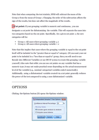
8. The p-value of Levene's test is printed as ".000" (but should be read as p < 0.001 --
i.e., p very small), so we we reject the null of Levene's test and conclude that the
variance in mile time of athletes is significantly different than that of non-
athletes. This tells us that we should look at the "Equal variances not
assumed" row for the t-test (and corresponding confidence interval)
results. (If this test result had not been significant -- that is, if we had
observed p > α -- then we would have used the "Equal variances assumed" output.)
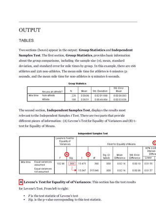
B t-test for Equality of Means provides the results for the actual Independent
Samples t Test. From left to right:
 t is the computed test statistic
 df is the degrees of freedom
 Sig (2-tailed) is the p-value corresponding to the given test statistic and
degrees of freedom
 Mean Difference is the difference between the sample means; it also
corresponds to the numerator of the test statistic
 Std. Error Difference is the standard error; it also corresponds to the
denominator of the test statistic
Note that the mean difference is calculated by subtracting the mean of the second
group from the mean of the first group. In this example, the mean mile time for
athletes was subtracted from the mean mile time for non-athletes (9:06 minus 6:51 =
02:14). The sign of the mean difference corresponds to the sign of the t value. The
positive t value in this example indicates that the mean mile time for the first group,
non-athletes, is significantly greater than the mean for the second group, athletes.
The associated p value is printed as ".000". Note that p-values are never actually
equal to 0; SPSS prints ".000" when the p-value is so small that it is hidden by
rounding error. (In this particular examples, the p-values are on the order of 10
-40
.)
C Confidence Interval of the Difference: This part of the t-test output
complements the significance test results. Typically, if the CI for the mean difference
contains 0, the results are not significant at the chosen significance level. In this
example, the 95% CI is [01:57, 02:32], which does not contain zero; this agrees with
the small p-value of the significance test.

9. DECISION AND CONCLUSIONS
Since p < .0001 is less than our chosen significance level α = 0.05, we can reject the
null hypothesis, and conclude that the that the mean mile time for athletes and non-
athletes is significantly different.
Based on the results, we can state the following:
 There was a significant difference in mean mile time between non-athletes
and athletes (t315.846
= 15.047, p < .001).
 The average mile time for athletes was 2 minutes and 14 seconds faster than
the average mile time for non-athletes.
Note: In your reports, you should never write that p=0.000, even if that is what
is in the SPSS output. Instead, use the mathematically correct statement that p <
0.001 (which basically says "p is very small").