Download as PDF, PPTX


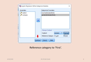


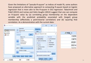

![The classification table provides the frequencies and percentages reflecting the degree
to which the model correctly and incorrectly predicts category membership on the
dependent variable. We see that 100%*23/(23+2) = 92% of cases that were observed
not terminate early were correctly predicted (by the model) to not terminate early. Of
the 20 cases observed to terminate early, 100%*15/(5+15) = 75% were correctly
predicted by the model to terminate early. [As you can see, sensitivity refers to
accuracy of the model in predicting target group membership, whereas specificity
refers to the accuracy of a model to predict non-target group membership.] The overall
classification accuracy based on the model was 84.4%.
3/29/2020 DR ATHAR KHAN 19](https://image.slidesharecdn.com/spssbinarylogisticregressiondemo1terminate-converted-200329160128/85/Binary-OR-Binomial-logistic-regression-19-320.jpg)
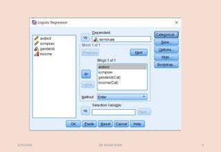
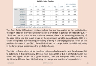
![The ‘Estimate’ column contains the regression coefficients. For each predictor, the
regression slope is the predicted change in the log odds of falling into the target group (as
compared to the reference group on the dependent variable) per one unit increase on
the predictor (controlling for the remaining predictors). [Note: A common misconception
is that the regression coefficient indicates the predicted change in probability of target
group membership per unit increase on the predictor – i.e., p(Y=1|X’s). This is WRONG!
The coefficient is the predicted change in log odds per unit increase on the predictor].
Nevertheless, you can generally interpret a positive regression coefficient as indicating
the probability (loosely speaking) of falling into the target group increases as a result of
increases on the predictor variable; and that a negative coefficient indicates that the
probability (again, loosely speaking) of target membership decreases with increases on
the predictor. If the regression coefficient = 0, this can be taken to indicate changes in the
probability of being in the target group as scores on the predictor increase.
3/29/2020 DR ATHAR KHAN 20](https://image.slidesharecdn.com/spssbinarylogisticregressiondemo1terminate-converted-200329160128/85/Binary-OR-Binomial-logistic-regression-20-320.jpg)
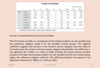
![▪ Avoidance of disclosure is a positive and significant (b=.3866, s.e.=.138, p=.005)
predictor of the probability of early termination, with the OR indicating that for
every one unit increase on this predictor the odds of early termination change by a
factor of 1.472 (meaning the odds are increasing).
▪ Symptom severity is a negative and significant (b=-.3496, s.e.=.137, p=.010)
predictor of the probability of early termination. The OR indicates that for every
one unit increment on the predictor, the odds of terminating increase by a factor of
.705 (meaning that the odds are decreasing).
▪ Genderid is a non-significant predictor of early termination (b=-1.5079, s.e.=.0956,
p=.115). [Had the predictor been significant, then the negative coefficient would be
taken as an indicator that females (coded 1) are less likely to terminate early than
males.]
3/29/2020 DR ATHAR KHAN 22](https://image.slidesharecdn.com/spssbinarylogisticregressiondemo1terminate-converted-200329160128/85/Binary-OR-Binomial-logistic-regression-22-320.jpg)


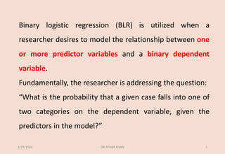
Binary logistic regression can be used to model the relationship between predictor variables and a binary dependent variable. The document discusses using logistic regression to predict the likelihood of clients terminating counseling early based on gender, income level, avoidance of disclosure, and symptom severity. The full model was statistically significant and correctly classified 84.4% of cases. Avoidance of disclosure and symptom severity significantly predicted early termination, while gender and income level were not significant predictors.