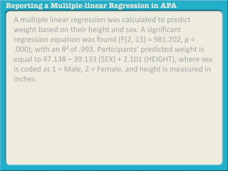
A multiple linear regression was calculated to predict weight based on height and sex. The regression equation was significant and height and sex were significant predictors of weight, explaining 99.3% of the variance. Participants' predicted weight is equal to 47.138 - 39.133 (sex) + 2.101 (height), where height is measured in inches and sex is coded as 0 for female and 1 for male.

1. Reporting a Multiple Linear
Regression in APA Format
Amit Sharma
Associate Professor
Dept. of Pharmacy Practice
ISF COLLEGE OF PHARMACY
Ghal Kalan, Ferozpur GT Road, MOGA, 142001, Punjab
Mobile: 09646755140, 09418783145
Phone: No. 01636-650150, 650151
Website: - www.isfcp.org

2. Note – the examples in this presentation come from,
Cronk, B. C. (2012). How to Use SPSS Statistics: A
Step-by-step Guide to Analysis and Interpretation.
Pyrczak Pub.

3. Here’s the template:

4. DV = Dependent Variable
IV = Independent Variable

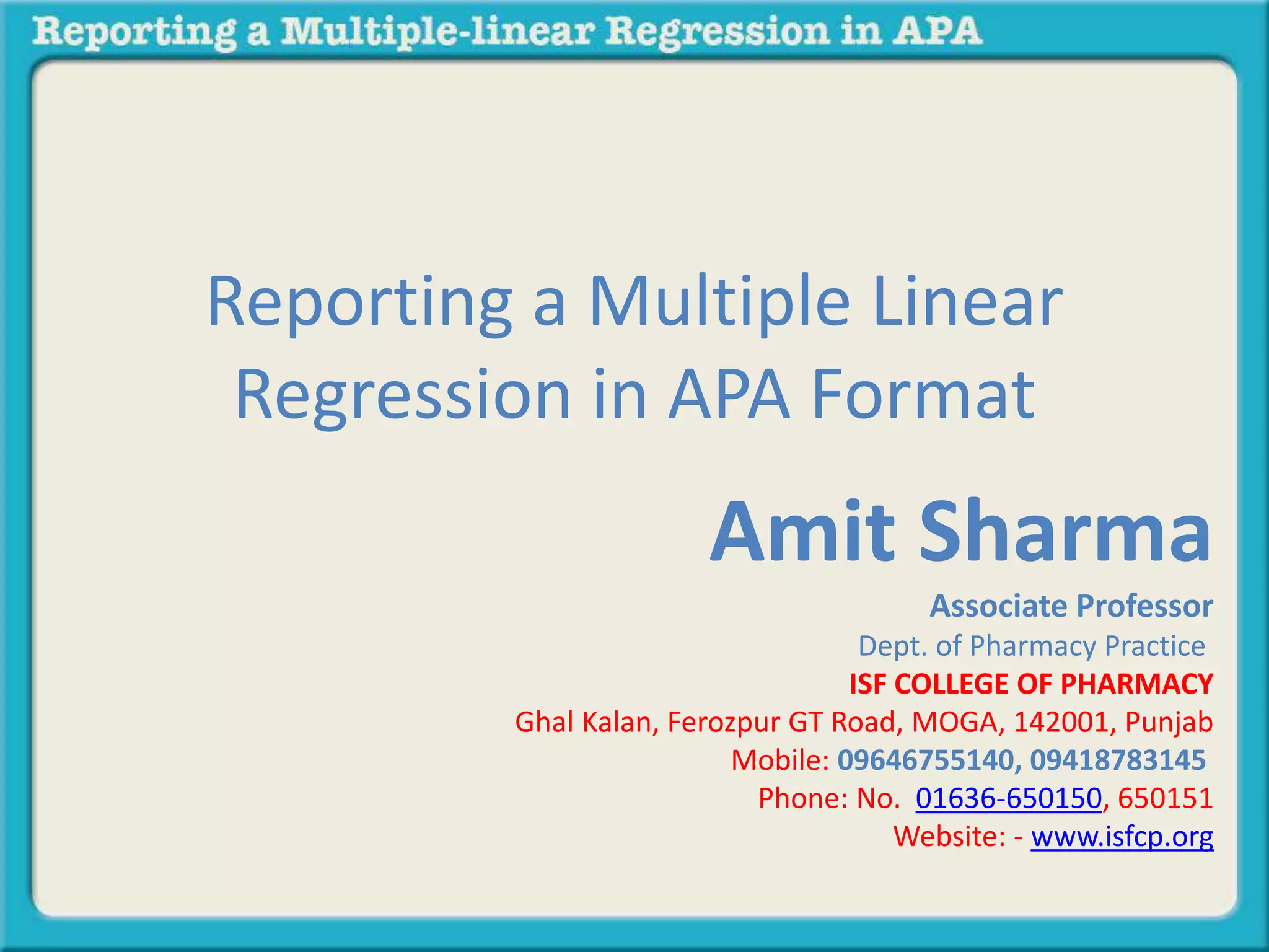
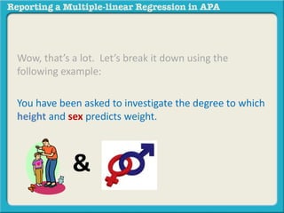
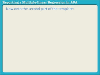
5. DV = Dependent Variable
IV = Independent Variable
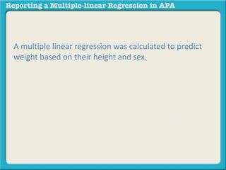
A multiple linear regression was calculated to predict
[DV] based on [IV1] and [IV2]. A significant regression
equation was found (F(_,__) = ___.___, p < .___), with
an R2 of .___. Participants’ predicted [DV] is equal to
__.___ – __.___ (IV1) + _.___ (IV2), where [IV1] is coded
or measured as _____________, and [IV2] is coded or
measured as __________. Object of measurement
increased _.__ [DV unit of measure] for each [IV1 unit
of measure] and _.__ for each [IV2 unit of measure].
Both [IV1] and [IV2] were significant predictors of [DV].

6. Wow, that’s a lot. Let’s break it down using the
following example:

7. Wow, that’s a lot. Let’s break it down using the
following example:
You have been asked to investigate the degree to which
height and sex predicts weight.

8. Wow, that’s a lot. Let’s break it down using the
following example:
You have been asked to investigate the degree to which
height and sex predicts weight.

9. Wow, that’s a lot. Let’s break it down using the
following example:
You have been asked to investigate the degree to which
height and sex predicts weight.
&

10. Wow, that’s a lot. Let’s break it down using the
following example:
You have been asked to investigate the degree to which
height and sex predicts weight.
&

11. Let’s begin with the first part of the template:

12. A multiple linear regression was calculated to predict
[DV] based on their [IV1] and [IV2].

13. A multiple linear regression was calculated to predict
[DV] based on their [IV1] and [IV2].
You have been asked to investigate the degree to which
height and sex predicts weight.

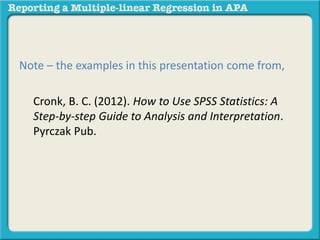
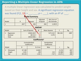
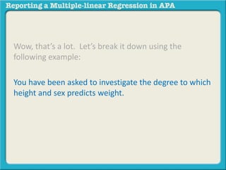
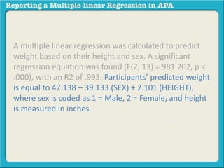
14. A multiple linear regression was calculated to predict
weight based on their [IV1] and [IV2].
You have been asked to investigate the degree to which
height and sex predicts weight.

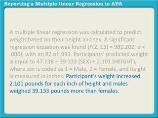
15. A multiple linear regression was calculated to predict
weight based on their height and [IV2].
You have been asked to investigate the degree to which
height and sex predicts weight.

16. A multiple linear regression was calculated to predict
weight based on their height and sex.
You have been asked to investigate the degree to which
height and sex predicts weight.

17. Now onto the second part of the template:

18. A multiple linear regression was calculated to predict weight
based on their height and sex. A significant regression equation
was found (F(_,__) = __.___, p < .___), with an R2 of .____.

19. A multiple linear regression was calculated to predict weight
based on their height and sex. A significant regression equation
was found (F(_,__) = ___.___, p < .___), with an R2 of .___.

20. A multiple linear regression was calculated to predict weight
based on their height and sex. A significant regression equation
was found (F(_,__) = ___.___, p < .___), with an R2 of .___.
Here’s the output:

21. A multiple linear regression was calculated to predict weight
based on their height and sex. A significant regression equation
was found (F(_,__) = ___.___, p < .___), with an R2 of .___.
Model Summary
Model R R Square
Adjusted
R Square
Std. Error of
the Estimate
1 .997a .993 .992 2.29571
ANOVAa
Model Sum of Squares df Mean Squares F Sig.
1. Regression
Residual
Total
10342.424
68.514
10410.938
2
13
15
5171.212
5.270
981.202 .000a
Coefficientsa
Model
Unstandardized
Coefficients
Standardized
Coefficients
t Sig.B St. Error Beta
1. (Constant)
Height
Sex
47.138
2.101
-39.133
14.843
.198
1.501
.312
-7.67
-3.176
10.588
-25.071
.007
.000
.000

22. A multiple linear regression was calculated to predict weight
based on their height and sex. A significant regression equation
was found (F(2,__) = ___.___, p < .___), with an R2 of .___.
Model Summary
Model R R Square
Adjusted
R Square
Std. Error of
the Estimate
1 .997a .993 .992 2.29571
ANOVAa
Model Sum of Squares df Mean Squares F Sig.
1. Regression
Residual
Total
10342.424
68.514
10410.938
2
13
15
5171.212
5.270
981.202 .000a
Coefficientsa
Model
Unstandardized
Coefficients
Standardized
Coefficients
t Sig.B St. Error Beta
1. (Constant)
Height
Sex
47.138
2.101
-39.133
14.843
.198
1.501
.312
-7.67
-3.176
10.588
-25.071
.007
.000
.000

23. A multiple linear regression was calculated to predict weight
based on their height and sex. A significant regression equation
was found (F(2, 13) = ___.___, p < .___), with an R2 of .___.
Model Summary
Model R R Square
Adjusted
R Square
Std. Error of
the Estimate
1 .997a .993 .992 2.29571
ANOVAa
Model Sum of Squares df Mean Squares F Sig.
1. Regression
Residual
Total
10342.424
68.514
10410.938
2
13
15
5171.212
5.270
981.202 .000a
Coefficientsa
Model
Unstandardized
Coefficients
Standardized
Coefficients
t Sig.B St. Error Beta
1. (Constant)
Height
Sex
47.138
2.101
-39.133
14.843
.198
1.501
.312
-7.67
-3.176
10.588
-25.071
.007
.000
.000

24. A multiple linear regression was calculated to predict weight
based on their height and sex. A significant regression equation
was found (F(2, 13) = 981.202, p < .___), with an R2 of .___.
Model Summary
Model R R Square
Adjusted
R Square
Std. Error of
the Estimate
1 .997a .993 .992 2.29571
ANOVAa
Model Sum of Squares df Mean Squares F Sig.
1. Regression
Residual
Total
10342.424
68.514
10410.938
2
13
15
5171.212
5.270
981.202 .000a
Coefficientsa
Model
Unstandardized
Coefficients
Standardized
Coefficients
t Sig.B St. Error Beta
1. (Constant)
Height
Sex
47.138
2.101
-39.133
14.843
.198
1.501
.312
-7.67
-3.176
10.588
-25.071
.007
.000
.000

25. A multiple linear regression was calculated to predict weight
based on their height and sex. A significant regression equation
was found (F(2, 13) = 981.202, p < .000), with an R2 of .___.
Model Summary
Model R R Square
Adjusted
R Square
Std. Error of
the Estimate
1 .997a .993 .992 2.29571
ANOVAa
Model Sum of Squares df Mean Squares F Sig.
1. Regression
Residual
Total
10342.424
68.514
10410.938
2
13
15
5171.212
5.270
981.202 .000a
Coefficientsa
Model
Unstandardized
Coefficients
Standardized
Coefficients
t Sig.B St. Error Beta
1. (Constant)
Height
Sex
47.138
2.101
-39.133
14.843
.198
1.501
.312
-7.67
-3.176
10.588
-25.071
.007
.000
.000

26. A multiple linear regression was calculated to predict weight
based on their height and sex. A significant regression equation
was found (F(2, 13) = 981.202, p < .000), with an R2 of .993.
Model Summary
Model R R Square
Adjusted
R Square
Std. Error of
the Estimate
1 .997a .993 .992 2.29571
ANOVAa
Model Sum of Squares df Mean Squares F Sig.
1. Regression
Residual
Total
10342.424
68.514
10410.938
2
13
15
5171.212
5.270
981.202 .000a
Coefficientsa
Model
Unstandardized
Coefficients
Standardized
Coefficients
t Sig.B St. Error Beta
1. (Constant)
Height
Sex
47.138
2.101
-39.133
14.843
.198
1.501
.312
-7.67
-3.176
10.588
-25.071
.007
.000
.000

27. A multiple linear regression was calculated to predict weight
based on their height and sex. A significant regression equation
was found (F(2, 13) = 981.202, p < .000), with an R2 of .993.
Now for the next part of the template:

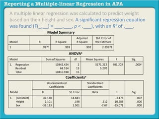
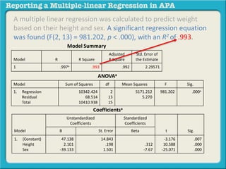
28. A multiple linear regression was calculated to predict weight
based on their height and sex. A significant regression equation
was found (F(2, 13) = 981.202, p < .000), with an R2 of .993.
Participants’ predicted [DV] is equal to __.___ + __.___ (IV2) +
_.___ (IV1), where [IV2] is coded or measured as _____________,
and [IV1] is coded or measured __________.

29. A multiple linear regression was calculated to predict weight
based on their height and sex. A significant regression equation
was found (F(2, 13) = 981.202, p < .000), with an R2 of .993.
Participants’ predicted [DV] is equal to __.___ + __.___ (IV1) +
_.___ (IV2), where [IV1] is coded or measured as _____________,
and [IV2] is coded or measured __________.
ANOVAa
Model Sum of Squares df Mean Squares F Sig.
1. Regression
Residual
Total
10342.424
68.514
10410.938
2
13
15
5171.212
5.270
981.202 .000a
Coefficientsa
Model
Unstandardized
Coefficients
Standardized
Coefficients
t Sig.B St. Error Beta
1. (Constant)
Height
Sex
47.138
2.101
-39.133
14.843
.198
1.501
.312
-7.67
-3.176
10.588
-25.071
.007
.000
.000

30. A multiple linear regression was calculated to predict weight
based on their height and sex. A significant regression equation
was found (F(2, 13) = 981.202, p < .000), with an R2 of .993.
Participants’ predicted [DV] is equal to __.___ + __.___ (IV1) +
_.___ (IV2), where [IV1] is coded or measured as _____________,
and [IV2] is coded or measured __________.
Coefficientsa
Model
Unstandardized
Coefficients
Standardized
Coefficients
t Sig.B St. Error Beta
1. (Constant)
Height
Sex
47.138
2.101
-39.133
14.843
.198
1.501
.312
-7.67
-3.176
10.588
-25.071
.007
.000
.000
Independent Variable1: Height
Independent Variable2: Sex
Dependent Variable: Weight

31. A multiple linear regression was calculated to predict weight
based on their height and sex. A significant regression equation
was found (F(2, 13) = 981.202, p < .000), with an R2 of .993.
Participants’ predicted weight is equal to __.___ + __.___ (IV1) +
_.___ (IV2), where [IV1] is coded or measured as _____________,
and [IV2] is coded or measured __________.
Coefficientsa
Model
Unstandardized
Coefficients
Standardized
Coefficients
t Sig.B St. Error Beta
1. (Constant)
Height
Sex
47.138
2.101
-39.133
14.843
.198
1.501
.312
-7.67
-3.176
10.588
-25.071
.007
.000
.000
Independent Variable1: Height
Independent Variable2: Sex
Dependent Variable: Weight

32. A multiple linear regression was calculated to predict weight
based on their height and sex. A significant regression equation
was found (F(2, 13) = 981.202, p < .000), with an R2 of .993.
Participants’ predicted weight is equal to 47.138 + __.___ (IV1) +
_.___ (IV2), where [IV1] is coded or measured as _____________,
and [IV2] is coded or measured __________.
Coefficientsa
Model
Unstandardized
Coefficients
Standardized
Coefficients
t Sig.B St. Error Beta
1. (Constant)
Height
Sex
47.138
2.101
-39.133
14.843
.198
1.501
.312
-7.67
-3.176
10.588
-25.071
.007
.000
.000
Independent Variable1: Height
Independent Variable2: Sex
Dependent Variable: Weight

33. A multiple linear regression was calculated to predict weight
based on their height and sex. A significant regression equation
was found (F(2, 13) = 981.202, p < .000), with an R2 of .993.
Participants’ predicted weight is equal to 47.138 – 39.133 (IV1) +
_.___ (IV1), where [IV1] is coded or measured as _____________,
and [IV2] is coded or measured __________.
Coefficientsa
Model
Unstandardized
Coefficients
Standardized
Coefficients
t Sig.B St. Error Beta
1. (Constant)
Height
Sex
47.138
2.101
-39.133
14.843
.198
1.501
.312
-7.67
-3.176
10.588
-25.071
.007
.000
.000
Independent Variable1: Height
Independent Variable2: Sex
Dependent Variable: Weight

34. A multiple linear regression was calculated to predict weight
based on their height and sex. A significant regression equation
was found (F(2, 13) = 981.202, p < .000), with an R2 of .993.
Participants’ predicted weight is equal to 47.138 – 39.133 (SEX) +
_.___ (IV1), where [IV1] is coded or measured as _____________,
and [IV2] is coded or measured __________.
Coefficientsa
Model
Unstandardized
Coefficients
Standardized
Coefficients
t Sig.B St. Error Beta
1. (Constant)
Height
Sex
47.138
2.101
-39.133
14.843
.198
1.501
.312
-7.67
-3.176
10.588
-25.071
.007
.000
.000
Independent Variable1: Height
Independent Variable2: Sex
Dependent Variable: Weight

35. A multiple linear regression was calculated to predict weight
based on their height and sex. A significant regression equation
was found (F(2, 13) = 981.202, p < .000), with an R2 of .993.
Participants’ predicted weight is equal to 47.138 – 39.133 (SEX) +
2.101 (IV1), where [IV1] is coded or measured as _____________,
and [IV2] is coded or measured __________.
Coefficientsa
Model
Unstandardized
Coefficients
Standardized
Coefficients
t Sig.B St. Error Beta
1. (Constant)
Height
Sex
47.138
2.101
-39.133
14.843
.198
1.501
.312
-7.67
-3.176
10.588
-25.071
.007
.000
.000
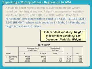
Independent Variable1: Height
Independent Variable2: Sex
Dependent Variable: Weight

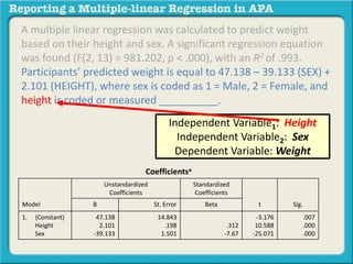
36. A multiple linear regression was calculated to predict weight
based on their height and sex. A significant regression equation
was found (F(2, 13) = 981.202, p < .000), with an R2 of .993.
Participants’ predicted weight is equal to 47.138 – 39.133 (SEX) +
2.101 (HEIGHT), where [IV1] is coded or measured as
_____________, and [IV2] is coded or measured __________.
Coefficientsa
Model
Unstandardized
Coefficients
Standardized
Coefficients
t Sig.B St. Error Beta
1. (Constant)
Height
Sex
47.138
2.101
-39.133
14.843
.198
1.501
.312
-7.67
-3.176
10.588
-25.071
.007
.000
.000
Independent Variable1: Height
Independent Variable2: Sex
Dependent Variable: Weight

37. A multiple linear regression was calculated to predict weight
based on their height and sex. A significant regression equation
was found (F(2, 13) = 981.202, p < .000), with an R2 of .993.
Participants’ predicted weight is equal to 47.138 – 39.133 (SEX) +
2.101 (HEIGHT), where sex is coded or measured as
_____________, and [IV2] is coded or measured __________.
Coefficientsa
Model
Unstandardized
Coefficients
Standardized
Coefficients
t Sig.B St. Error Beta
1. (Constant)
Height
Sex
47.138
2.101
-39.133
14.843
.198
1.501
.312
-7.67
-3.176
10.588
-25.071
.007
.000
.000
Independent Variable1: Height
Independent Variable2: Sex
Dependent Variable: Weight

38. A multiple linear regression was calculated to predict weight
based on their height and sex. A significant regression equation
was found (F(2, 13) = 981.202, p < .000), with an R2 of .993.
Participants’ predicted weight is equal to 47.138 – 39.133 (SEX) +
2.101 (HEIGHT), where sex is coded as 1 = Male, 2 = Female, and
[IV2] is coded or measured __________.
Coefficientsa
Model
Unstandardized
Coefficients
Standardized
Coefficients
t Sig.B St. Error Beta
1. (Constant)
Height
Sex
47.138
2.101
-39.133
14.843
.198
1.501
.312
-7.67
-3.176
10.588
-25.071
.007
.000
.000
Independent Variable1: Height
Independent Variable2: Sex
Dependent Variable: Weight

39. A multiple linear regression was calculated to predict weight
based on their height and sex. A significant regression equation
was found (F(2, 13) = 981.202, p < .000), with an R2 of .993.
Participants’ predicted weight is equal to 47.138 – 39.133 (SEX) +
2.101 (HEIGHT), where sex is coded as 1 = Male, 2 = Female, and
height is coded or measured __________.
Coefficientsa
Model
Unstandardized
Coefficients
Standardized
Coefficients
t Sig.B St. Error Beta
1. (Constant)
Height
Sex
47.138
2.101
-39.133
14.843
.198
1.501
.312
-7.67
-3.176
10.588
-25.071
.007
.000
.000
Independent Variable1: Height
Independent Variable2: Sex
Dependent Variable: Weight

40. A multiple linear regression was calculated to predict weight
based on their height and sex. A significant regression equation
was found (F(2, 13) = 981.202, p < .000), with an R2 of .993.
Participants’ predicted weight is equal to 47.138 – 39.133 (SEX) +
2.101 (HEIGHT), where sex is coded as 1 = Male, 2 = Female, and
height is measured in inches.
Coefficientsa
Model
Unstandardized
Coefficients
Standardized
Coefficients
t Sig.B St. Error Beta
1. (Constant)
Height
Sex
47.138
2.101
-39.133
14.843
.198
1.501
.312
-7.67
-3.176
10.588
-25.071
.007
.000
.000
Independent Variable1: Height
Independent Variable2: Sex
Dependent Variable: Weight

41. A multiple linear regression was calculated to predict weight
based on their height and sex. A significant regression equation
was found (F(2, 13) = 981.202, p < .000), with an R2 of .993.
Participants’ predicted weight is equal to 47.138 – 39.133 (SEX) +
2.101 (HEIGHT), where sex is coded as 1 = Male, 2 = Female, and
height is measured in inches.
Coefficientsa
Model
Unstandardized
Coefficients
Standardized
Coefficients
t Sig.B St. Error Beta
1. (Constant)
Height
Sex
47.138
2.101
-39.133
14.843
.198
1.501
.312
-7.67
-3.176
10.588
-25.071
.007
.000
.000
Independent Variable1: Height
Independent Variable2: Sex
Dependent Variable: Weight

42. Now for the second to last portion of the template:

43. A multiple linear regression was calculated to predict
weight based on their height and sex. A significant
regression equation was found (F(2, 13) = 981.202, p <
.000), with an R2 of .993. Participants’ predicted weight is
equal to 47.138 – 39.133 (SEX) + 2.101 (HEIGHT), where sex
is coded as 1 = Male, 2 = Female, and height is measured in
inches.

44. A multiple linear regression was calculated to predict
weight based on their height and sex. A significant
regression equation was found (F(2, 13) = 981.202, p <
.000), with an R2 of .993. Participants’ predicted weight is
equal to 47.138 – 39.133 (SEX) + 2.101 (HEIGHT), where sex
is coded as 1 = Male, 2 = Female, and height is measured in
inches. Object of measurement increased _.__ [DV unit of
measure] for each [IV1 unit of measure] and _.__ for each
[IV2 unit of measure].

45. A multiple linear regression was calculated to predict
weight based on their height and sex. A significant
regression equation was found (F(2, 13) = 981.202, p <
.000), with an R2 of .993. Participants’ predicted weight is
equal to 47.138 – 39.133 (SEX) + 2.101 (HEIGHT), where sex
is coded as 1 = Male, 2 = Female, and height is measured in
inches. Object of measurement increased _.__ [DV unit of
measure] for each [IV1 unit of measure] and _.__ for each
[IV2 unit of measure].
Coefficientsa
Model
Unstandardized
Coefficients
Standardized
Coefficients
t Sig.B St. Error Beta
1. (Constant)
Height
Sex
47.138
2.101
-39.133
14.843
.198
1.501
.312
-7.67
-3.176
10.588
-25.071
.007
.000
.000

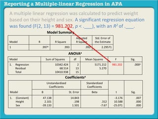
46. A multiple linear regression was calculated to predict
weight based on their height and sex. A significant
regression equation was found (F(2, 13) = 981.202, p <
.000), with an R2 of .993. Participants’ predicted weight is
equal to 47.138 – 39.133 (SEX) + 2.101 (HEIGHT), where sex
is coded as 1 = Male, 2 = Female, and height is measured in
inches. Participant’s weight increased _.__ [DV unit of
measure] for each [IV1 unit of measure] and _.__ for each
[IV2 unit of measure].
Coefficientsa
Model
Unstandardized
Coefficients
Standardized
Coefficients
t Sig.B St. Error Beta
1. (Constant)
Height
Sex
47.138
2.101
-39.133
14.843
.198
1.501
.312
-7.67
-3.176
10.588
-25.071
.007
.000
.000

47. A multiple linear regression was calculated to predict
weight based on their height and sex. A significant
regression equation was found (F(2, 13) = 981.202, p <
.000), with an R2 of .993. Participants’ predicted weight is
equal to 47.138 – 39.133 (SEX) + 2.101 (HEIGHT), where sex
is coded as 1 = Male, 2 = Female, and height is measured in
inches. Participant’s weight increased 2.101 [DV unit of
measure] for each [IV1 unit of measure] and _.__ for each
[IV2 unit of measure].
Coefficientsa
Model
Unstandardized
Coefficients
Standardized
Coefficients
t Sig.B St. Error Beta
1. (Constant)
Height
Sex
47.138
2.101
-39.133
14.843
.198
1.501
.312
-7.67
-3.176
10.588
-25.071
.007
.000
.000

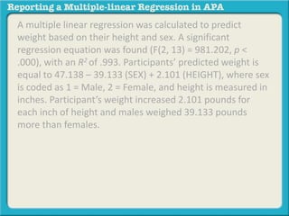
48. A multiple linear regression was calculated to predict
weight based on their height and sex. A significant
regression equation was found (F(2, 13) = 981.202, p <
.000), with an R2 of .993. Participants’ predicted weight is
equal to 47.138 – 39.133 (SEX) + 2.101 (HEIGHT), where sex
is coded as 1 = Male, 2 = Female, and height is measured in
inches. Participant’s weight increased 2.101 pounds for
each [IV1 unit of measure] and _.__ for each [IV2 unit of
measure].
Coefficientsa
Model
Unstandardized
Coefficients
Standardized
Coefficients
t Sig.B St. Error Beta
1. (Constant)
Height
Sex
47.138
2.101
-39.133
14.843
.198
1.501
.312
-7.67
-3.176
10.588
-25.071
.007
.000
.000

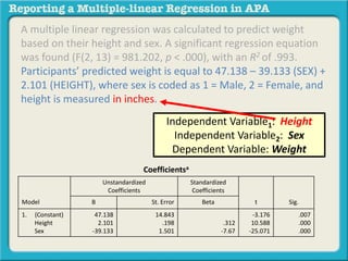
49. A multiple linear regression was calculated to predict
weight based on their height and sex. A significant
regression equation was found (F(2, 13) = 981.202, p <
.000), with an R2 of .993. Participants’ predicted weight is
equal to 47.138 – 39.133 (SEX) + 2.101 (HEIGHT), where sex
is coded as 1 = Male, 2 = Female, and height is measured in
inches. Participant’s weight increased 2.101 pounds for
each inch of height and _.__ for each [IV2 unit of measure].
Coefficientsa
Model
Unstandardized
Coefficients
Standardized
Coefficients
t Sig.B St. Error Beta
1. (Constant)
Height
Sex
47.138
2.101
-39.133
14.843
.198
1.501
.312
-7.67
-3.176
10.588
-25.071
.007
.000
.000

50. A multiple linear regression was calculated to predict
weight based on their height and sex. A significant
regression equation was found (F(2, 13) = 981.202, p <
.000), with an R2 of .993. Participants’ predicted weight is
equal to 47.138 – 39.133 (SEX) + 2.101 (HEIGHT), where sex
is coded as 1 = Male, 2 = Female, and height is measured in
inches. Participant’s weight increased 2.101 pounds for
each inch of height and males weighed 39.133 pounds
more than females.
Coefficientsa
Model
Unstandardized
Coefficients
Standardized
Coefficients
t Sig.B St. Error Beta
1. (Constant)
Height
Sex
47.138
2.101
-39.133
14.843
.198
1.501
.312
-7.67
-3.176
10.588
-25.071
.007
.000
.000

51. Finally, the last part of the template:

52. A multiple linear regression was calculated to predict
weight based on their height and sex. A significant
regression equation was found (F(2, 13) = 981.202, p <
.000), with an R2 of .993. Participants’ predicted weight is
equal to 47.138 – 39.133 (SEX) + 2.101 (HEIGHT), where sex
is coded as 1 = Male, 2 = Female, and height is measured in
inches. Participant’s weight increased 2.101 pounds for
each inch of height and males weighed 39.133 pounds
more than females.

53. A multiple linear regression was calculated to predict
weight based on their height and sex. A significant
regression equation was found (F(2, 13) = 981.202, p <
.000), with an R2 of .993. Participants’ predicted weight is
equal to 47.138 – 39.133 (SEX) + 2.101 (HEIGHT), where sex
is coded as 1 = Male, 2 = Female, and height is measured in
inches. Participant’s weight increased 2.101 pounds for
each inch of height and males weighed 39.133 pounds
more than females. Both [IV1] and [IV2] were significant
predictors of [DV].

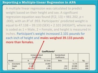
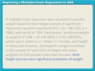
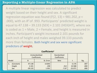
54. A multiple linear regression was calculated to predict
weight based on their height and sex. A significant
regression equation was found (F(2, 13) = 981.202, p <
.000), with an R2 of .993. Participants’ predicted weight is
equal to 47.138 – 39.133 (SEX) + 2.101 (HEIGHT), where sex
is coded as 1 = Male, 2 = Female, and height is measured in
inches. Participant’s weight increased 2.101 pounds for
each inch of height and males weighed 39.133 pounds
more than females. Both [IV1] and [IV2] were significant
predictors of [DV].
Coefficientsa
Model
Unstandardized
Coefficients
Standardized
Coefficients
t Sig.B St. Error Beta
1. (Constant)
Height
Sex
47.138
2.101
-39.133
14.843
.198
1.501
.312
-7.67
-3.176
10.588
-25.071
.007
.000
.000

55. A multiple linear regression was calculated to predict
weight based on their height and sex. A significant
regression equation was found (F(2, 13) = 981.202, p <
.000), with an R2 of .993. Participants’ predicted weight is
equal to 47.138 – 39.133 (SEX) + 2.101 (HEIGHT), where sex
is coded as 1 = Male, 2 = Female, and height is measured in
inches. Participant’s weight increased 2.101 pounds for
each inch of height and males weighed 39.133 pounds
more than females. Both height and [IV2] were significant
predictors of [DV].
Coefficientsa
Model
Unstandardized
Coefficients
Standardized
Coefficients
t Sig.B St. Error Beta
1. (Constant)
Height
Sex
47.138
2.101
-39.133
14.843
.198
1.501
.312
-7.67
-3.176
10.588
-25.071
.007
.000
.000

56. A multiple linear regression was calculated to predict
weight based on their height and sex. A significant
regression equation was found (F(2, 13) = 981.202, p <
.000), with an R2 of .993. Participants’ predicted weight is
equal to 47.138 – 39.133 (SEX) + 2.101 (HEIGHT), where sex
is coded as 1 = Male, 2 = Female, and height is measured in
inches. Participant’s weight increased 2.101 pounds for
each inch of height and males weighed 39.133 pounds
more than females. Both height and sex were significant
predictors of [DV].
Coefficientsa
Model
Unstandardized
Coefficients
Standardized
Coefficients
t Sig.B St. Error Beta
1. (Constant)
Height
Sex
47.138
2.101
-39.133
14.843
.198
1.501
.312
-7.67
-3.176
10.588
-25.071
.007
.000
.000

57. A multiple linear regression was calculated to predict
weight based on their height and sex. A significant
regression equation was found (F(2, 13) = 981.202, p <
.000), with an R2 of .993. Participants’ predicted weight is
equal to 47.138 – 39.133 (SEX) + 2.101 (HEIGHT), where sex
is coded as 1 = Male, 2 = Female, and height is measured in
inches. Participant’s weight increased 2.101 pounds for
each inch of height and males weighed 39.133 pounds
more than females. Both height and sex were significant
predictors of [DV].
. Coefficientsa
Model
Unstandardized
Coefficients
Standardized
Coefficients
t Sig.B St. Error Beta
1. (Constant)
Height
Sex
47.138
2.101
-39.133
14.843
.198
1.501
.312
-7.67
-3.176
10.588
-25.071
.007
.000
.000

58. A multiple linear regression was calculated to predict
weight based on their height and sex. A significant
regression equation was found (F(2, 13) = 981.202, p <
.000), with an R2 of .993. Participants’ predicted weight is
equal to 47.138 – 39.133 (SEX) + 2.101 (HEIGHT), where sex
is coded as 1 = Male, 2 = Female, and height is measured in
inches. Participant’s weight increased 2.101 pounds for
each inch of height and males weighed 39.133 pounds
more than females. Both height and sex were significant
predictors of weight.
. Coefficientsa
Model
Unstandardized
Coefficients
Standardized
Coefficients
t Sig.B St. Error Beta
1. (Constant)
Height
Sex
47.138
2.101
-39.133
14.843
.198
1.501
.312
-7.67
-3.176
10.588
-25.071
.007
.000
.000

59. And there you are:

60. A multiple linear regression was calculated to predict
weight based on their height and sex. A significant
regression equation was found (F(2, 13) = 981.202, p <
.000), with an R2 of .993. Participants’ predicted weight
is equal to 47.138 – 39.133 (SEX) + 2.101 (HEIGHT),
where sex is coded as 1 = Male, 2 = Female, and height
is measured in inches. Object of measurement
increased 2.101 pounds for each inch of height and
males weighed 39.133 pounds more than females.
Both height and sex were significant predictors.

61. A multiple linear regression was calculated to predict
weight based on their height and sex. A significant
regression equation was found (F(2, 13) = 981.202, p <
.000), with an R2 of .993. Participants’ predicted weight
is equal to 47.138 – 39.133 (SEX) + 2.101 (HEIGHT),
where sex is coded as 1 = Male, 2 = Female, and height
is measured in inches. Object of measurement
increased 2.101 pounds for each inch of height and
males weighed 39.133 pounds more than females.
Both height and sex were significant predictors.

62. A multiple linear regression was calculated to predict
weight based on their height and sex. A significant
regression equation was found (F(2, 13) = 981.202, p <
.000), with an R2 of .993. Participants’ predicted weight
is equal to 47.138 – 39.133 (SEX) + 2.101 (HEIGHT),
where sex is coded as 1 = Male, 2 = Female, and height
is measured in inches. Object of measurement
increased 2.101 pounds for each inch of height and
males weighed 39.133 pounds more than females.
Both height and sex were significant predictors.

63. A multiple linear regression was calculated to predict
weight based on their height and sex. A significant
regression equation was found (F(2, 13) = 981.202, p <
.000), with an R2 of .993. Participants’ predicted weight
is equal to 47.138 – 39.133 (SEX) + 2.101 (HEIGHT),
where sex is coded as 1 = Male, 2 = Female, and height
is measured in inches. Participant’s weight increased
2.101 pounds for each inch of height and males
weighed 39.133 pounds more than females. Both
height and sex were significant predictors.

64. A multiple linear regression was calculated to predict
weight based on their height and sex. A significant
regression equation was found (F(2, 13) = 981.202, p <
.000), with an R2 of .993. Participants’ predicted weight
is equal to 47.138 – 39.133 (SEX) + 2.101 (HEIGHT),
where sex is coded as 1 = Male, 2 = Female, and height
is measured in inches. Participant’s weight increased
2.101 pounds for each inch of height and males
weighed 39.133 pounds more than females. Both
height and sex were significant predictors of weight.

65. A multiple linear regression was calculated to predict
weight based on their height and sex. A significant
regression equation was found (F(2, 13) = 981.202, p <
.000), with an R2 of .993. Participants’ predicted weight
is equal to 47.138 – 39.133 (SEX) + 2.101 (HEIGHT),
where sex is coded as 1 = Male, 2 = Female, and height
is measured in inches. Participant’s weight increased
2.101 pounds for each inch of height and males
weighed 39.133 pounds more than females. Both
height and sex were significant predictors of weight.