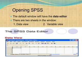
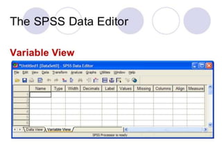
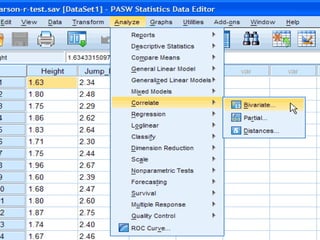
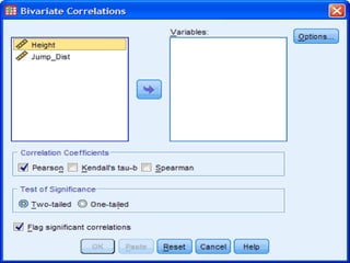
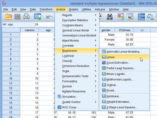
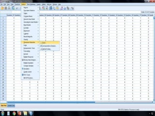
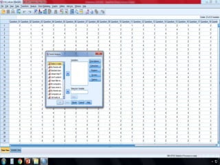
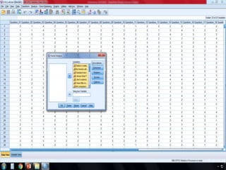
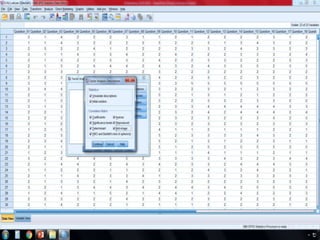
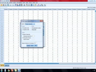
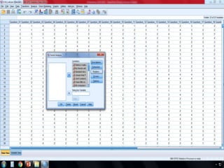
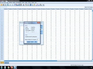
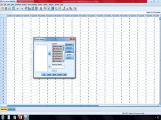
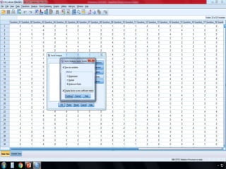
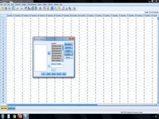
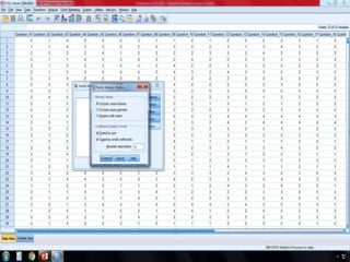
SPSS is a statistical software package used for interactive or programmed data analysis. It can perform complex data analysis and statistics with simple commands. Originally called the Statistical Package for the Social Sciences when it was first created in 1968, SPSS is now owned by IBM. The default window in SPSS contains a data editor with two sheets - the data view sheet displays raw data while the variable view sheet defines metadata for each variable. SPSS allows users to easily enter, clean, manage and analyze data to derive useful information for making informed decisions.
In this ppt the viewer will able to know about Epi Info- An Statistical Software. Epi Info is statistical software for epidemiology developed by Centers for Disease Control and Prevention (CDC) in Atlanta, Georgia (US). Epi Info has been in existence for over 20 years and is currently available for Microsoft Windows, Android and iOS, along with a web and cloud version. The program allows for electronic survey creation, data entry, and analysis. Within the analysis module, analytic routines include t-tests, ANOVA, nonparametric statistics, cross tabulations and stratification with estimates of odds ratios, risk ratios, and risk differences, logistic regression (conditional and unconditional), survival analysis (Kaplan Meier and Cox proportional hazard), and analysis of complex survey data.
Portion explained:
1. Epi Info Software
2. History of Epi Info Software
3. Features of Epi Info Software
4. Release history of Epi Info Software
Binary Logistic Regression Classification makes use of one or more predictor variables that may be either continuous or categorical to predict target variable classes. This technique identifies important factors impacting the target variable and also the nature of the relationship between each of these factors and the dependent variable. It is useful in the analysis of multiple factors influencing an outcome, or other classification where there two possible outcomes.
Applications of statistics in medical Research and HealthrMuhammadNafees42
This will help you to understand the applications of basic statistics.The application of stat in medical health and research.
#nafeesupdates
#nafeesmedicos
Statistical Package for Social Science (SPSS)sspink
This presentation includes the introduction of SPSS is basic features of Spss, how to input data manually, descriptive statistics and how to perform t-test, Anova and Chi-Square.
U3 IP.sav
MKTG420_U3IP.doc
Unit 3 Individual Project 1
MACROBUTTON DoFieldClick Type your Name Here
American Intercontinental University
MACROBUTTON DoFieldClick Type your Paper Title
Project Type: MKTG420 Unit 3 Individual Project
MACROBUTTON DoFieldClick Date of Submission
Abstract
This is a single paragraph, no indentation is required. The next page will be an abstract; “a brief, comprehensive summary of the contents of the article; it allows the readers to survey the contents of an article quickly” (Publication Manual, 2010). The length of this abstract should be 35-50 words (2-3 sentences). NOTE: the abstract must be on page 2 and the body of the paper will begin on page 3.
MACROBUTTON DoFieldClick Type your Paper Title
Introduction
Remember to always indent the first line of a paragraph (use the tab key). The introduction should be short (2-3 sentences). The margins, font size, spacing, and font type (italics or plain) are set in APA format. While you may change the names of the headings and subheadings, do not change the font.
Part 1: Research background on the scales
Introduce the concept and be sure to indent the first line of the paragraph. Provide background on each of the 4 scales (assurance, empathy, reliability and responsiveness), not limited to a simple definition but as a measurement that aids marketers. Discuss how the questions in the survey are transformed into "scales" (also called "factors"). In other studies using SERVQUAL, how many and what types of respondents were included? Part 1 of the Individual Project should be 1 page in length. Be sure to cite your resources.
Part 1: Concept of Scales/Factors
Introduce the concept and be sure to indent the first line of the paragraph.
Part 1: SERVQUAL Samples
Introduce the concept and be sure to indent the first line of the paragraph.
Part 2: (Full-Text Research) Service Quality and Segmentation
Introduce the concept and be sure to indent the first line of the paragraph. Connect information from at least 3 articles. Do not write and overview or critique of the articles. Synthesize and connect the information contained to develop a solid understanding of how service quality and segmentation are related. Part 2 of the Individual Project should be 2 pages in length and should be predominately from at least three articles in AIU's full-text databases. Be sure to cite your resources.
Part 3: Null/Hypo 1, ANOVA, Decision
Attached is a small set of data that has been collected from brand loyal customers of Store 1 and Store 2. Write out a Null hypothesis and an alternate hypothesis for each of the 4 aspects of service quality that are include in the analysis (assurance, empathy, reliability and responsiveness) to see if there is a difference between stores. Run 4 ANOVAs to test the Null hypotheses. State the decision for each of the tests.
Part 3: Null/Hypo 2, ANOVA, Decision
Write out a Null hypothesis and an alternate hypothesis ...
1Create a correlation table for the variables in our data set. (Us.docxjeanettehully
1
Create a correlation table for the variables in our data set. (Use analysis ToolPak function Correlation.)
a. Interpret the results.
What variables seem to be important in seeing if we pay males and females equally for equal work?
2
Below is a regression analysis for salary being predicted/explained by the other variables in our sample
(Mid,
age, ees, sr, raise, and deg variables.) (Note: since salary and compa are different ways of
expressing an employee’s salary, we do not want to have both used in the same regression.)
Ho: The regression equation is not significant.
Ha: The regression equation is significant.
Ho: The regression coefficient for each variable is not significant
Ha: The regression coefficient for each variable is significant
Sal
The analysis used Sal as the y (dependent variable) and
SUMMARY OUTPUT
mid, age, ees, sr, g, raise, and deg as the dependent
variables (entered as a range).
Regression Statistics
Multiple R
0.99215498
R Square
0.9843715
Adjusted R Square
0.98176675
Standard Error
2.59277631
Observations
50
ANOVA
df
SS
MS
F
Significance F
Regression
7
17783.7
2540.52
377.914
8.44043E-36
Residual
42
282.345
6.72249
Total
49
18066
Coefficients
Standard Error
t Stat
P-value
Lower 95%
Upper 95%
Lower 95.0%
Upper 95.0%
Intercept
-4.009
3.775
-1.062
0.294
-11.627
3.609
-11.627
3.609
Mid
1.220
0.030
40.674
0.000
1.159
1.280
1.159
1.280
Age
0.029
0.067
0.439
0.663
-0.105
0.164
-0.105
0.164
EES
-0.096
0.047
-2.020
0.050
-0.191
0.000
-0.191
0.000
SR
-0.074
0.084
-0.876
0.386
-0.244
0.096
-0.244
0.096
G
2.552
0.847
3.012
0.004
0.842
4.261
0.842
4.261
Raise
0.834
0.643
1.299
0.201
-0.462
2.131
-0.462
2.131
Deg
1.002
0.744
1.347
0.185
-0.500
2.504
-0.500
2.504
Interpretation:
Do you reject or not reject the regression null hypothesis?
Do you reject or not reject the null hypothesis for each variable?
What is the regression equation, using only significant variables if any exist?
What does result tell us about equal pay for equal work for males and females?
3
Perform a regression analysis using compa as the dependent variable and the same independent
variables as used in question 2.
Show the result, and interpret your findings by answering the same questions.
Note: be sure to include the appropriate hypothesis statements.
4
Based on all of your results to date, is gender a factor in the pay practices of this company?
Why or why not?
Which is the best variable to use in analyzing pay practices - salary or compa?
Why?
.
WEEK 6 – EXERCISES Enter your answers in the spaces pr.docxwendolynhalbert
WEEK 6 – EXERCISES
Enter your answers in the spaces provided. Save the file using your last name as the beginning of the file name (e.g., ruf_week6_exercises) and submit via “Assignments.” When appropriate,
show your work
. You can do the work by hand, scan/take a digital picture, and attach that file with your work.
1
.
A psychotherapist studied whether his clients self-disclosed more while sitting in an easy chair or lying down on a couch. All clients had previously agreed to allow the sessions to be videotaped for research purposes. The therapist randomly assigned 10 clients to each condition. The third session for each client was videotaped and an independent observer counted the clients’ disclosures. The therapist reported that “clients made more disclosures when sitting in easy chairs (
M
= 18.20) than when lying down on a couch (
M
= 14.31),
t
(18) = 2.84,
p
< .05, two-tailed.” Explain these results to a person who understands the
t
test for a single sample but knows nothing about the
t
test for independent means.
2.
A researcher compared the adjustment of adolescents who had been raised in homes that were either very structured or unstructured. Thirty adolescents from each type of family completed an adjustment inventory. The results are reported in the table below. Explain these results to a person who understands the
t
test for a single sample but knows nothing about the
t
test for independent means.
Means on Four Adjustment Scales for
Adolescents from Structured versus Unstructured Homes
Scale
Structured Homes
Unstructured Homes
t
Social Maturity
106.82
113.94
–1.07
School Adjustment
116.31
107.22
2.03*
Identity Development
89.48
94.32
1.93*
Intimacy Development
102.25
104.33
.32
______________________
*
p
< .05
3.
Do men with higher levels of a particular hormone show higher levels of assertiveness? Levels of this hormone were tested in 100 men. The top 10 and the bottom 10 were selected for the study. All participants took part in a laboratory simulation in which they were asked to role-play a person picking his car up from a mechanic’s shop. The simulation was videotaped and later judged by independent raters on each of four types of assertive statements made by the participant. The results are shown in the table below. Explain these results to a person who fully understands the
t
test for a single sample but knows nothing about the
t
test for independent means.
Mean Number of Assertive Statements
Type of Assertive Statement
Group
1
2
3
4
Men with High Levels
2.14
1.16
3.83
0.14
Men with Low Levels
1.21
1.32
2.33
0.38
t
3.81**
0.89
2.03*
0.58
______________________
*
p
< .05;
**
p
< 0.1
4.
A manager of a small store wanted to discourage shoplifters by putting signs around the store saying “Shoplifting is a crime!” However, he wanted to make sure this would not result in customers buying less. To test this, he displayed the signs every other W.
measurement and scaling is an important tool of research. by following the right and suitable scale will provide an appropriate result of research.this slide show will additionally provide the statistical testing for research measurement and scale.
Assignment 2 Tests of SignificanceThroughout this assignment yo.docxrock73
Assignment 2: Tests of Significance
Throughout this assignment you will review mock studies. You will needs to follow the directions outlined in the section using SPSS and decide whether there is significance between the variables. You will need to list the five steps of hypothesis testing (as covered in the lesson for Week 6) to see how every question should be formatted. You will complete all of the problems. Be sure to cut and past the appropriate test result boxes from SPSS under each problem and explain what you will do with your research hypotheses. All calculations should be coming from your SPSS. You will need to submit the SPSS output file to get credit for this assignment. This file will save as a .spv file and will need to be in a single file. In other words, you are not allowed to submit more than one output file for this assignment.
The five steps of hypothesis testing when using SPSS are as follows:
1. State your research hypothesis (H1) and null hypothesis (H0).
2. Identify your confidence interval (.05 or .01)
3. Conduct your analysis using SPSS.
4. Look for the valid score for comparison. This score is usually under ‘Sig 2-tail’ or ‘Sig. 2’. We will call this “p”.
5. Compare the two and apply the following rule:
a. If “p” is < or = confidence interval, than you reject the null.
Be sure to explain to the reader what this means in regards to your study. (Ex: will you recommend counseling services?)
* Be sure that your answers are clearly distinguishable. Perhaps you bold your font or use a different color.
ASSIGNMENT 2(200) WORD MINIUM
1. They allow us to see if our relationship is "statistically significant". (Remember that this only shows us that there is or is not a relationship but does NOT show us if it is big, small, or in-between.)
2. It let's us know if our findings can be generalized to the population which our sample was selected from and represents.
This week you will decide which test of significance you will use for your project. For this class your choices for tests will include one of the following:
· Chi-square
· t Test
· ANOVA
We will be using a process for hypothesis testing which outlines five steps researchers can follow to complete this process:
1. Write your research hypothesis (H1) and your null hypothesis (H0).
2. Identify and record your confidence interval. These are usually .05 (95%) or .01 (99%).
3. Complete the test using SPSS.
4. Identify the number under Sig. (2-tail). This will be represented by "p".
5. Compare the numbers in steps 2 and 4 and apply the following rule:
1. If p < or = confidence interval, than you reject the null hypothesis
Determine what to do with your null and explain this to your reader. Be sure to go beyond the phrase "reject or fail to reject the null" and explain how that impacts your research and best describes the relationship between variables.
TEST QUESTIONS-NEED FULL ANSWERS
Q1
Make up and discuss research examples corresponding to the various ...
Show drafts
volume_up
Empowering the Data Analytics Ecosystem: A Laser Focus on Value
The data analytics ecosystem thrives when every component functions at its peak, unlocking the true potential of data. Here's a laser focus on key areas for an empowered ecosystem:
1. Democratize Access, Not Data:
Granular Access Controls: Provide users with self-service tools tailored to their specific needs, preventing data overload and misuse.
Data Catalogs: Implement robust data catalogs for easy discovery and understanding of available data sources.
2. Foster Collaboration with Clear Roles:
Data Mesh Architecture: Break down data silos by creating a distributed data ownership model with clear ownership and responsibilities.
Collaborative Workspaces: Utilize interactive platforms where data scientists, analysts, and domain experts can work seamlessly together.
3. Leverage Advanced Analytics Strategically:
AI-powered Automation: Automate repetitive tasks like data cleaning and feature engineering, freeing up data talent for higher-level analysis.
Right-Tool Selection: Strategically choose the most effective advanced analytics techniques (e.g., AI, ML) based on specific business problems.
4. Prioritize Data Quality with Automation:
Automated Data Validation: Implement automated data quality checks to identify and rectify errors at the source, minimizing downstream issues.
Data Lineage Tracking: Track the flow of data throughout the ecosystem, ensuring transparency and facilitating root cause analysis for errors.
5. Cultivate a Data-Driven Mindset:
Metrics-Driven Performance Management: Align KPIs and performance metrics with data-driven insights to ensure actionable decision making.
Data Storytelling Workshops: Equip stakeholders with the skills to translate complex data findings into compelling narratives that drive action.
Benefits of a Precise Ecosystem:
Sharpened Focus: Precise access and clear roles ensure everyone works with the most relevant data, maximizing efficiency.
Actionable Insights: Strategic analytics and automated quality checks lead to more reliable and actionable data insights.
Continuous Improvement: Data-driven performance management fosters a culture of learning and continuous improvement.
Sustainable Growth: Empowered by data, organizations can make informed decisions to drive sustainable growth and innovation.
By focusing on these precise actions, organizations can create an empowered data analytics ecosystem that delivers real value by driving data-driven decisions and maximizing the return on their data investment.
Explore our comprehensive data analysis project presentation on predicting product ad campaign performance. Learn how data-driven insights can optimize your marketing strategies and enhance campaign effectiveness. Perfect for professionals and students looking to understand the power of data analysis in advertising. for more details visit: https://bostoninstituteofanalytics.org/data-science-and-artificial-intelligence/
Adjusting primitives for graph : SHORT REPORT / NOTESSubhajit Sahu
Graph algorithms, like PageRank Compressed Sparse Row (CSR) is an adjacency-list based graph representation that is
Multiply with different modes (map)
1. Performance of sequential execution based vs OpenMP based vector multiply.
2. Comparing various launch configs for CUDA based vector multiply.
Sum with different storage types (reduce)
1. Performance of vector element sum using float vs bfloat16 as the storage type.
Sum with different modes (reduce)
1. Performance of sequential execution based vs OpenMP based vector element sum.
2. Performance of memcpy vs in-place based CUDA based vector element sum.
3. Comparing various launch configs for CUDA based vector element sum (memcpy).
4. Comparing various launch configs for CUDA based vector element sum (in-place).
Sum with in-place strategies of CUDA mode (reduce)
1. Comparing various launch configs for CUDA based vector element sum (in-place).
Levelwise PageRank with Loop-Based Dead End Handling Strategy : SHORT REPORT ...Subhajit Sahu
Abstract — Levelwise PageRank is an alternative method of PageRank computation which decomposes the input graph into a directed acyclic block-graph of strongly connected components, and processes them in topological order, one level at a time. This enables calculation for ranks in a distributed fashion without per-iteration communication, unlike the standard method where all vertices are processed in each iteration. It however comes with a precondition of the absence of dead ends in the input graph. Here, the native non-distributed performance of Levelwise PageRank was compared against Monolithic PageRank on a CPU as well as a GPU. To ensure a fair comparison, Monolithic PageRank was also performed on a graph where vertices were split by components. Results indicate that Levelwise PageRank is about as fast as Monolithic PageRank on the CPU, but quite a bit slower on the GPU. Slowdown on the GPU is likely caused by a large submission of small workloads, and expected to be non-issue when the computation is performed on massive graphs.
Levelwise PageRank with Loop-Based Dead End Handling Strategy : SHORT REPORT ...
Spss software
1. What is SPSS?
“Statistical Package for the Social Science”
One of the most popular statistical
packages which can perform highly
complex data and analysis with simple
instructions.
2. SPSS Inc. founded in 1968
2009 acquired by IBM
SPSS is now owned b y IBM
4. Opening SPSS
The default window will have the data editor
There are two sheets in the window:
1. Data view 2. Variable view
5.
6. Variable View window
Name
The first character of the variable
name must be alphabetic
less than 64 characters.
Spaces are NOT allowed.
7. Type
The two basic types of variables that you will use are
numeric and string.
8. Width
Width allows you to determine the number of
characters SPSS will allow to be entered for
the variable
9. Decimals
Number of decimals
It has to be less than or equal to 16
3.14159265
10. Label
Describing the variable
You can write characters with spaces up
to 256 characters
11. Values(coding)
This is used and to suggest which
numbers represent which categories
when the variable represents a
category
12. Defining the value labels
Click the cell in the values column
For the value, and the label, you can put up to 60
characters.
After defining the values click add and then click OK.
13. MISSING
Missing value:
• Not captured in the data set: errors in
feeding ...
•Empty value - No value in the population
15. Sample Questionnaire
Gender : Male / Female
Age : below 25/ 26-35/ 36-45/ 46-55
Category : student / Faculty / research scholars
How do you come to know about this
program(multiple choice)
Mail / WhatsApp/ friends/website
17. Saving the data
To save the data file -click ‘file’ and click
‘save as.’ You can save the file in different
forms by clicking “Save as type.”
Click
18. Opening the sample data
Open ‘Employee data.sav’ from the SPSS
Go to “File,” “Open,” and Click Data
30. Leave the Model: set as "Alpha", which represents
Cronbach's alpha in SPSS Statistics. If you want to
provide a name for the scale, enter it in the Scale label.
31.
32. Click the CONTINUE button,
Click the OK button to generate the output.
35. Cronbach's Alpha
.00-1.0
00 = no consistency in measurement (negative
consistency)
1.0= perfect consistency in measurement(positive
consistency)
.70= 70% of the variance in score is reliable
(acceptable level .7)
39. Hypotheses
Ha = Male and female have same academic score.
Ho = Male and female don’t have same academic score.
40. Rule of Thumb
If sig. value is > .05 = Accept Ho
If sig. value is < .05 = Accept Ha
41. Conditions :
dependent variable should be measured on a
interval or ratio scale.
Independent variable should consist of two
categorical group.(Nominal )
There needs to be homogeneity of variances.
Levene’s test for homogeneity
42.
43.
44.
45.
46. OUTPUT
If the levene’s sig value > .05 t-test should be based on
equal variance.
47.
48. Paired Samples t Test
Detect a difference between the mean of two
dependent variables.
Eg :
Measure the employees performance before and after
training .
49. Conditions
Dependent variable should be interval or ratio scale.
Two groups(dependent)
Normality
Homogeneity of variances
53. The sig. value is .000
which is < .05
Reject Ho
There is a significant difference between before and
after training.
We can conclude that the training program is effective
56. Eg
How strongly the sales are related with
advertising expenditure?
Work experience and their output.
Exam performance and preparation
time.
Online test score and students work
experience.
65. ANOVA is used to determine whether
there are any significant differences
between the means of more than two
independent groups.
understand whether exam performance
differed based on their community type
( urban, rural, semi-urban)
66. Conditions :
Dependent variable should be
measured at the interval or ratio
level.
Independent variable should consist
of three or more categorical group.
Normality
67.
68.
69.
70. Post hoc
ANOVA result will tell us whether there is a difference
among at least two of the group , but it will not tell us
which of the group exhibited this difference.
Post hoc help us to identify which group are different.
74. Exercise 1
Do students in each of the three
groups of community type have
similar academic score?
75. Two way ANOVA
SIGNIFICANT DIFFRENCE
BETWEEN TWO VARIABLES .
EXAMPLE
Scores – dependent
Age - Independent
Gender – Independent
76. Conditions :
Dependent variable should be ratio scale
Independent variables should be nominal
scale.
Two independent variable
Homogeneity (equality) of
variances(levene’s model)
77. Hypotheses
H1= Gender have no significant effect
on students academic score
H2= age have no significant effect on
score.
H3 = gender and age interaction have
no significant effect on score.
80. Displays overall mean,
means for each level of
duration, mean for each
level of modality and the
means for each
combination of duration by
modality (= the interaction
means).
Means
81. Levene’s test. This significant result means
the assumption of equal group variances
has not been met.
Output
82. In this case the analysis is not valid !.
Output
83.
84. Exercise : sample 3
Does the place of operations influences
ROCE?
Does the Industry type influences
ROCE?
97. It is used when we want to predict the value of a
variable(dependent) based on the value of another
variable.(independent).
Use multiple regression if independent variable are
more than one.
Example: How well can we predict a test score based
on work experience?
98. Conditions
variables should be measured at the interval or ratio
scale.
There needs to be a linear relationship between the
two variables(use scatter plot)
No significant outliers (observed data should not be
deviated from rest of the data).
One independent and one dependent variable.
99. Eg
Exam performance can be predicted based on revision
time.
Cigarette consumption can be predicted based on
smoking duration.
sales can be predicted based on ad.expenditure.
100.
101.
102.
103.
104. R is correlation value
R square = How much of the total variation in the
dependent variable can be explained by the
independent variable.
76.2% which is very large.
110. Cause and effect relationship
Eg you could use multiple regression to understand
whether exam performance can be predicted based on
revision time, lecture attendance and work exp.
111. It helps you to determine the overall fit (variance
explained) of the model .
Eg 2: sales can be predicted by sales men exp. And ad
exp.
112. Conditions
Dependent variable should be an interval scale.
You have two or more independent variables.
There needs to be a linear relationship between
independent and dependent variable.(scatter plot)
Your data must not show multicollinearity(R)
There should be no significant outliers
119. R, the multiple correlation coefficient,
R2 value ,which is the proportion of variance in the
dependent variable that can be explained by the
independent variables.
121. The table shows that the independent variables
statistically significantly predict the dependent
variable, F(4, 95) = 32.393, p < .0005 (i.e., the
regression model is a good fit of the data).
123. Exploratory Factor Analysis
Basic Concepts
What is Factor
Analysis?
The basic assumption of factor analysis is that for a
collection of observed variables there are a set
of underlying variables called factors (smaller than
the observed variables), that can explain the
interrelationships among those variables.
124. Exploratory Factor Analysis
Basic Concepts
Sample Size to Run a Factor
Analysis
10-15 Respondents per
variable
300 or more than 300 is a
good sample size
Run Kaiser-Meyer-Olkin
Measure of Sampling
Adequacy(KMO) test
125.
126.
127.
128.
129.
130.
131.
132.
133.
134.
135.
136.
137.
138.
139. KMO and Bartlett's Test
Kaiser-Meyer-Olkin Measure of Sampling
Adequacy. .930
Bartlett's Test of
Sphericity
Approx. Chi-
Square
19334.49
2
df 253
Sig. .000
Interpreting
Exploratory Factor Analysis Output
140. Communalities
Initial Extraction
Statiscs makes me cry 1.000 .435
My friends will think I'm stupid for not
being able to cope with SPSS
1.000 .414
Standard deviations excite me 1.000 .530
I dream that Pearson is attacking me with
correlation coefficients
1.000 .469
I don't understand statistics 1.000 .343
I have little experience of computers 1.000 .654
All computers hate me 1.000 .545
I have never been good at mathematics 1.000 .739
My friends are better at statistics than me 1.000 .484
Computers are useful only for playing
games
1.000 .335
I did badly at mathematics at school 1.000 .690
People try to tell you that SPSS makes
statistics easier to understand but it doesn't
1.000 .513
I worry that I will cause irreparable
damage because of my incompetenece with
computers
1.000 .536
Computers have minds of their own and
deliberately go wrong whenever I use them
1.000 .488
Computers are out to get me 1.000 .378
I weep openly at the mention of central
tendency
1.000 .487
I slip into a coma whenever I see an
equation
1.000 .683
SPSS always crashes when I try to use it 1.000 .597
Everybody looks at me when I use SPSS 1.000 .343
I can't sleep for thoughts of eigen vectors 1.000 .484
I wake up under my duvet thinking that I
am trapped under a normal distribtion
1.000 .550
My friends are better at SPSS than I am 1.000 .464
Interpreting
Exploratory
Factor Analysis
Output
142. Rotated Component Matrixa
Component
1 2 3 4
I have little experience of computers .800
SPSS always crashes when I try to use it .684
I worry that I will cause irreparable damage because
of my incompetence with computers
.647
All computers hate me .638
Computers have minds of their own and deliberately
go wrong whenever I use them
.579
Computers are useful only for playing games .550
Computers are out to get me .459
I can't sleep for thoughts of Eigen vectors .677
I wake up under my duvet thinking that I am trapped
under a normal distribution
.661
Standard deviations excite me -.567
People try to tell you that SPSS makes statistics easier
to understand but it doesn't
.473 .523
I dream that Pearson is attacking me with correlation
coefficients
.516
I weep openly at the mention of central tendency .514
Statiscs makes me cry .496
I don't understand statistics .429
I have never been good at mathematics .833
I slip into a coma whenever I see an equation .747
I did badly at mathematics at school .747
My friends are better at statistics than me .648
My friends are better at SPSS than I am .645
If I'm good at statistics my friends will think I'm a
nerd
.586
My friends will think I'm stupid for not being able to
cope with SPSS
.543
Everybody looks at me when I use SPSS .428
Extraction Method: Principal Component Analysis.
Rotation Method: Varimax with Kaiser Normalization.
Interpreting
Exploratory
Factor
Analysis
Output
143. Factors
Fear of
Compute
rs
Fear of
Statistics
Fear of
Maths
Peer
Evaluatio
n
I have little experience of computers .800
SPSS always crashes when I try to use it .684
I worry that I will cause irreparable damage because
of my incompetence with computers
.647
All computers hate me .638
Computers have minds of their own and deliberately
go wrong whenever I use them
.579
Computers are useful only for playing games .550
Computers are out to get me .459
I can't sleep for thoughts of Eigen vectors .677
I wake up under my duvet thinking that I am trapped
under a normal distribution
.661
Standard deviations excite me -.567
People try to tell you that SPSS makes statistics
easier to understand but it doesn't
.473 .523
I dream that Pearson is attacking me with
correlation coefficients
.516
I weep openly at the mention of central tendency .514
Statiscs makes me cry .496
I don't understand statistics .429
I have never been good at mathematics .833
I slip into a coma whenever I see an equation .747
I did badly at mathematics at school .747
My friends are better at statistics than me .648
My friends are better at SPSS than I am .645
If I'm good at statistics my friends will think I'm a
nerd
.586
My friends will think I'm stupid for not being able to .543
Interpreting
Exploratory
Factor
Analysis
Output