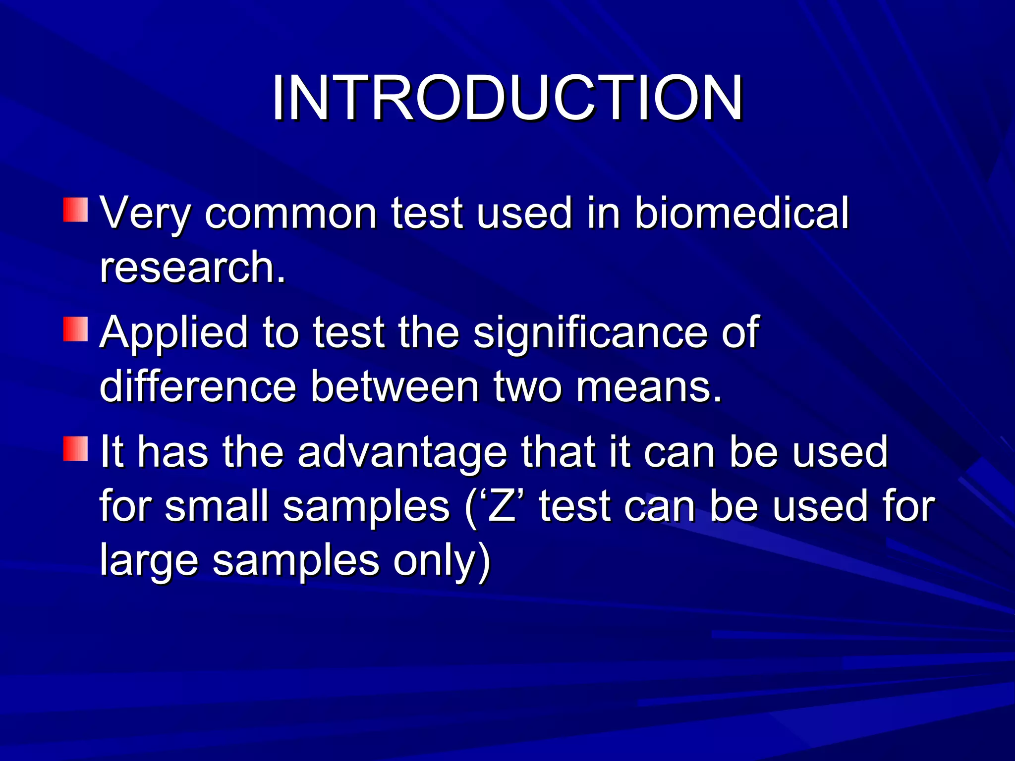
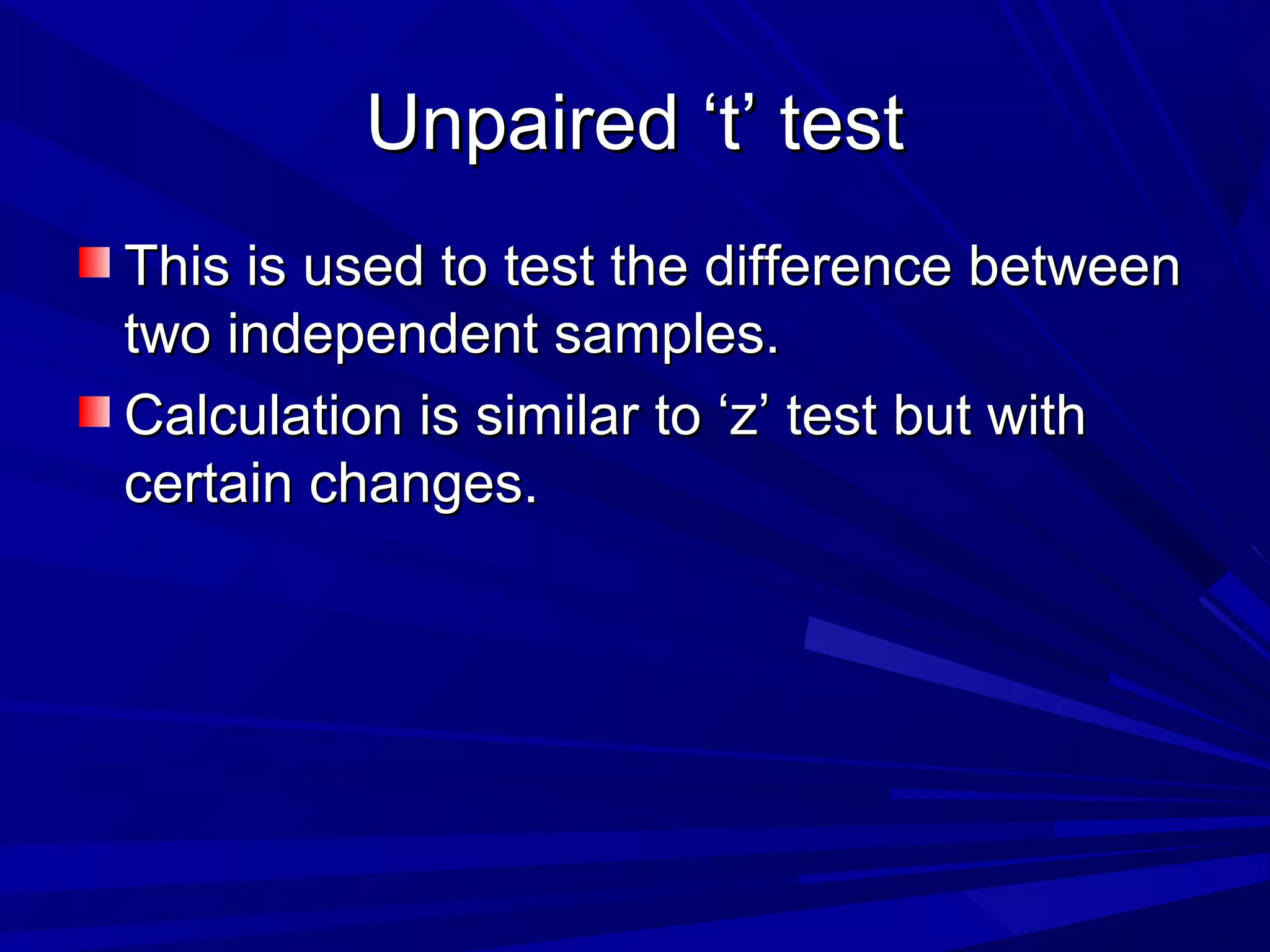
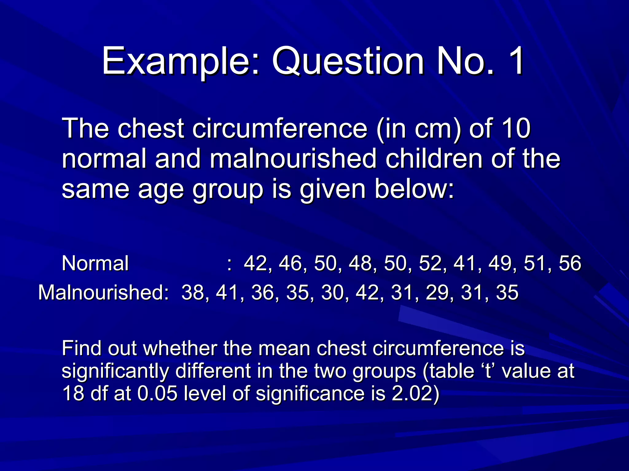
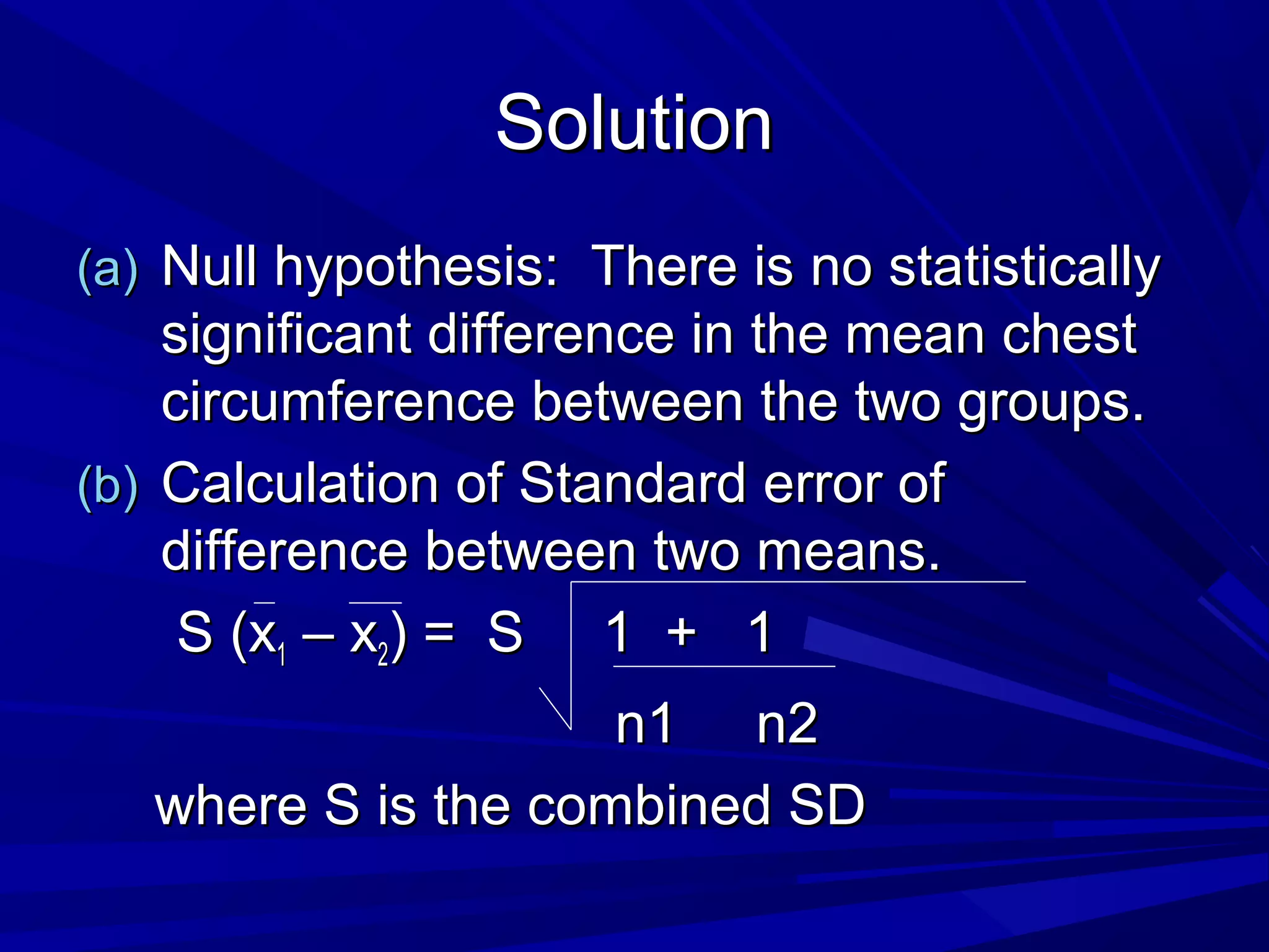
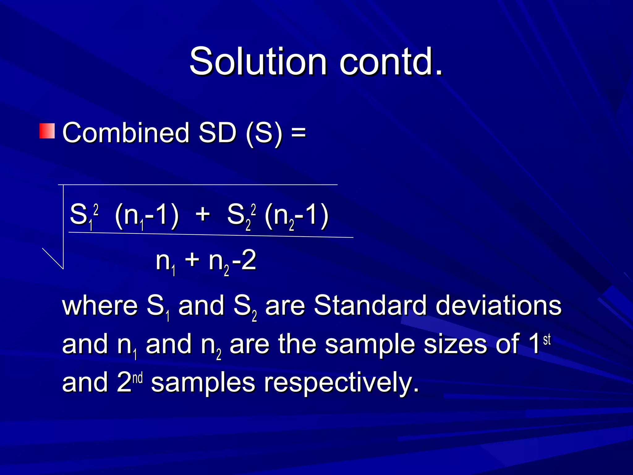
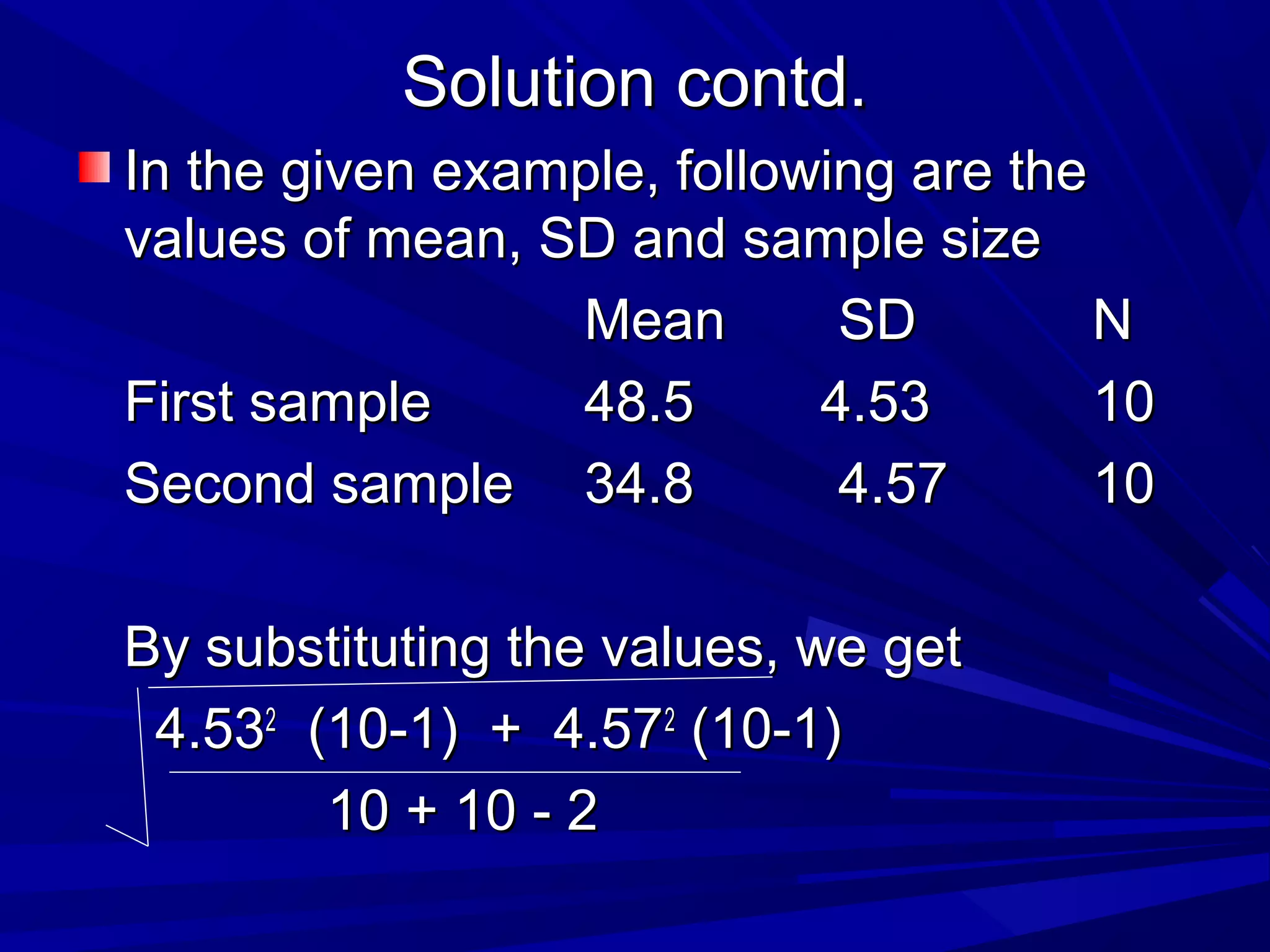
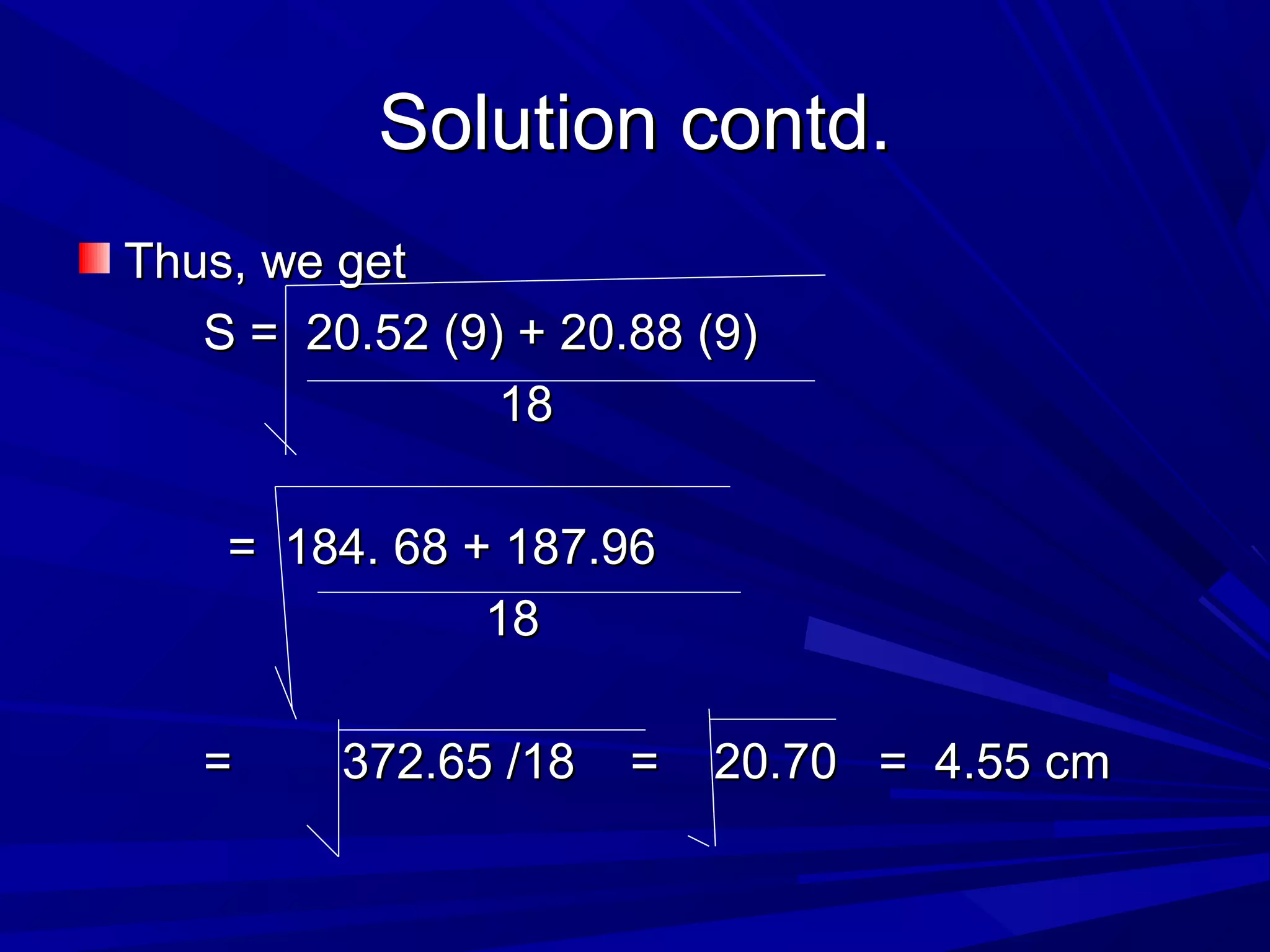
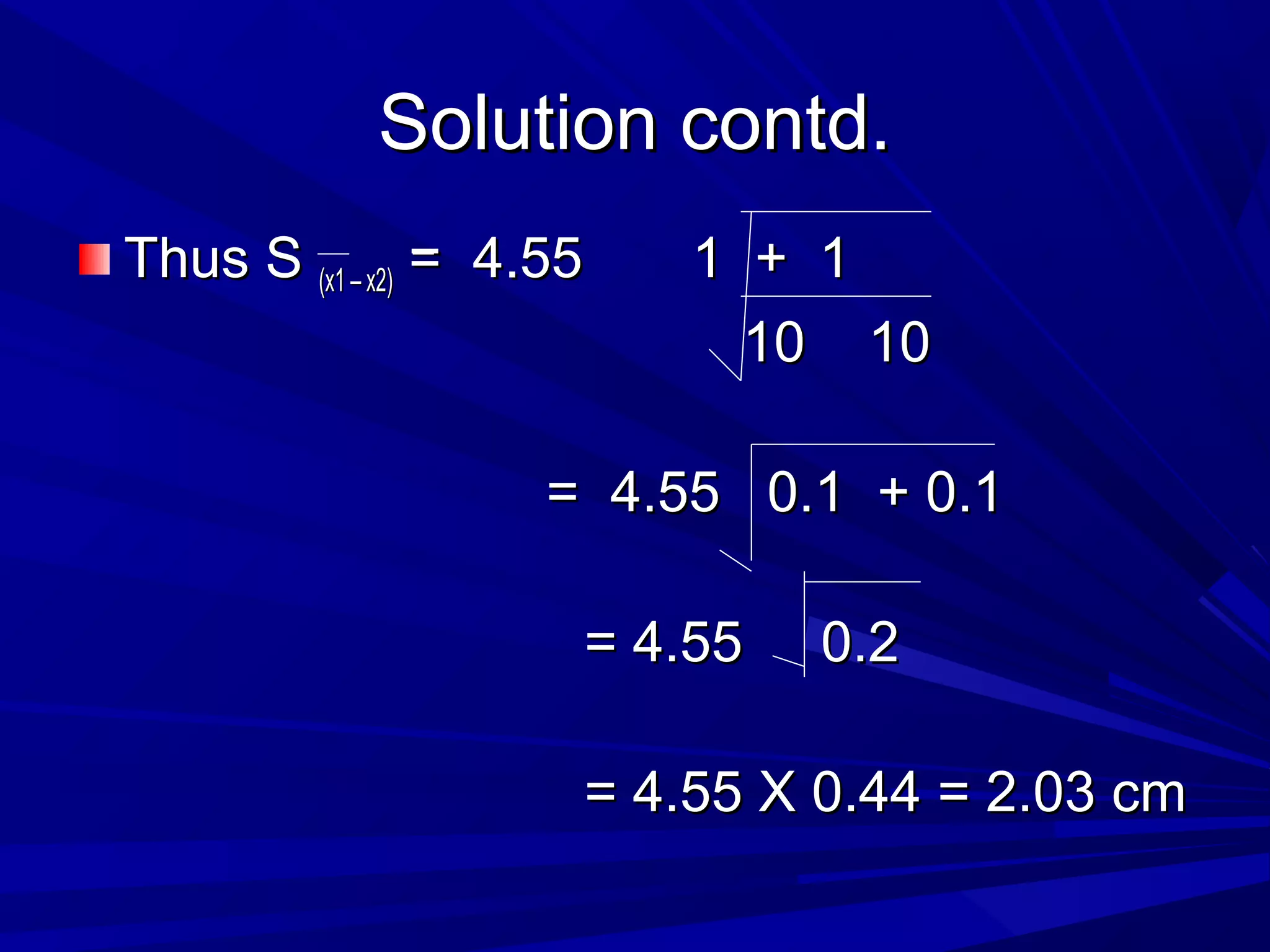
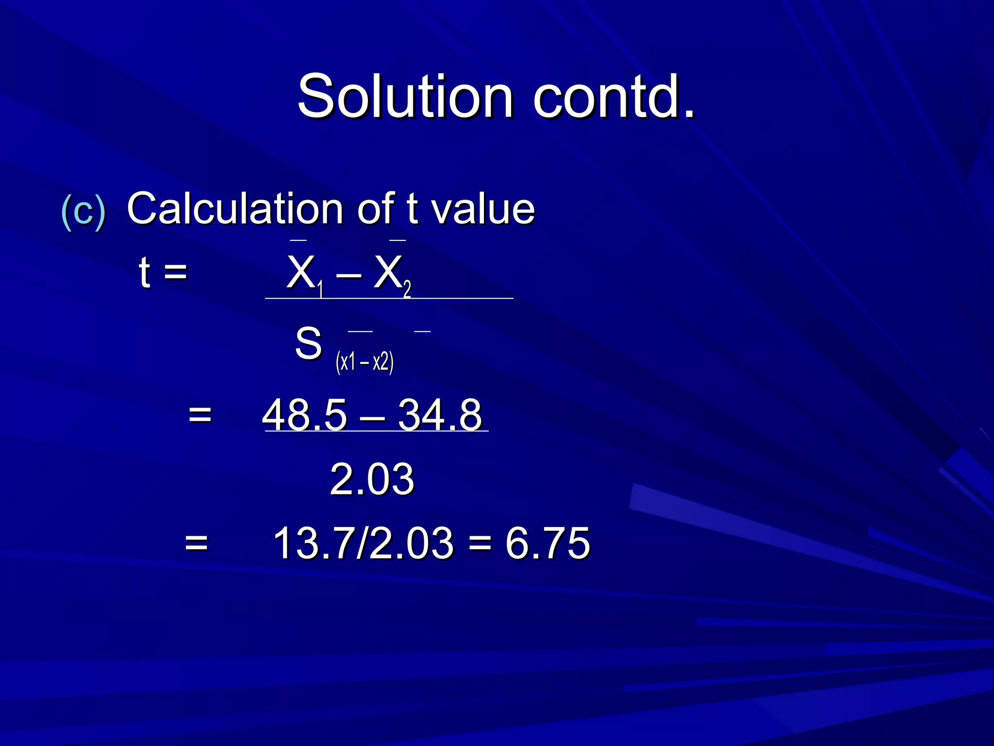
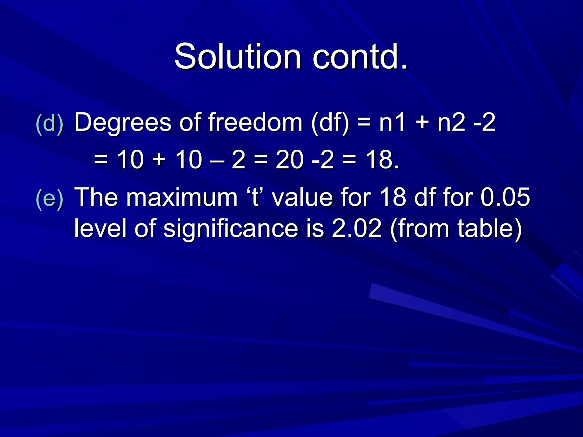
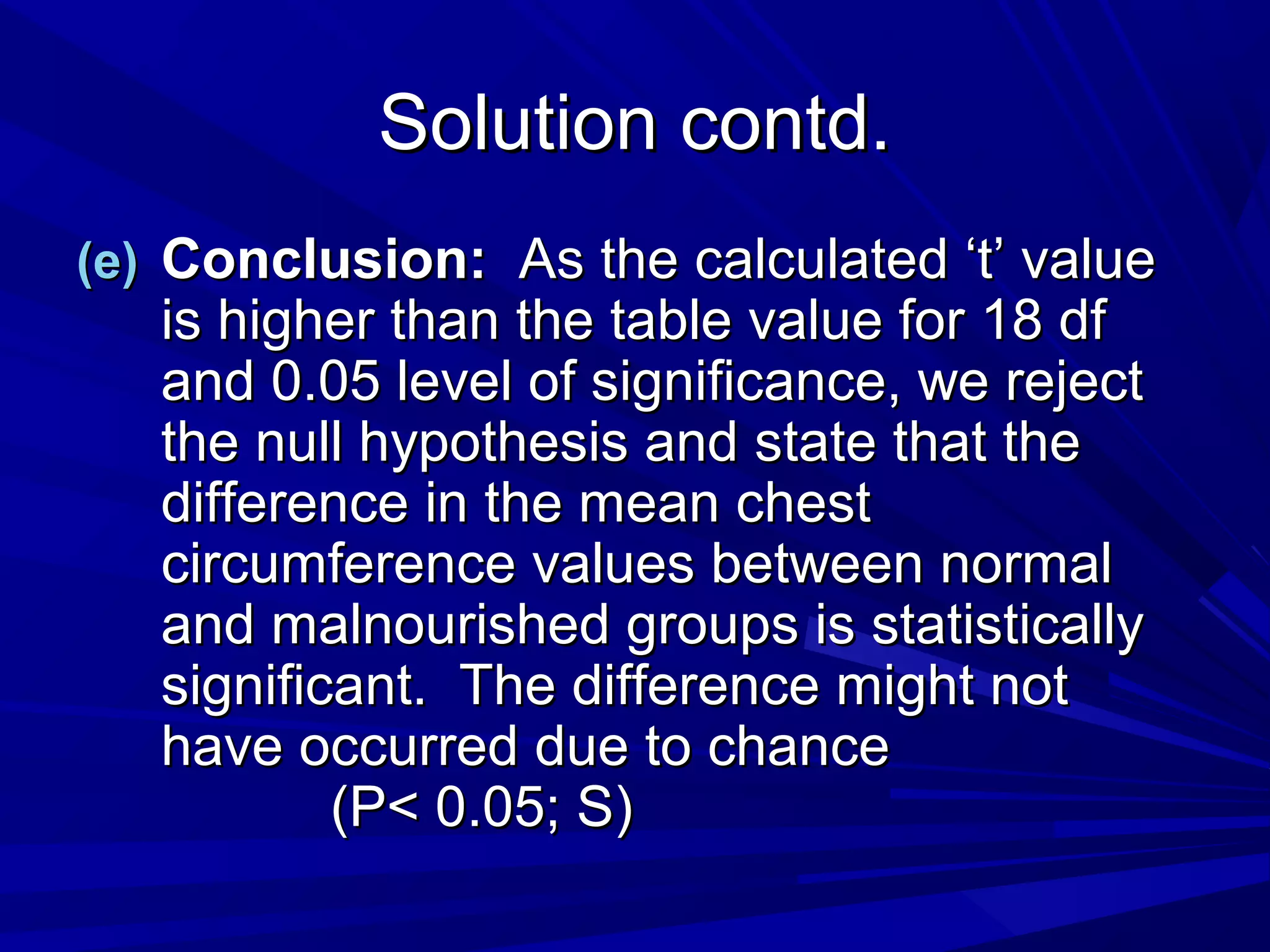
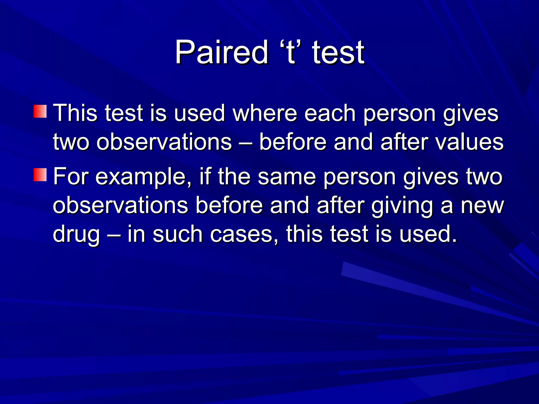
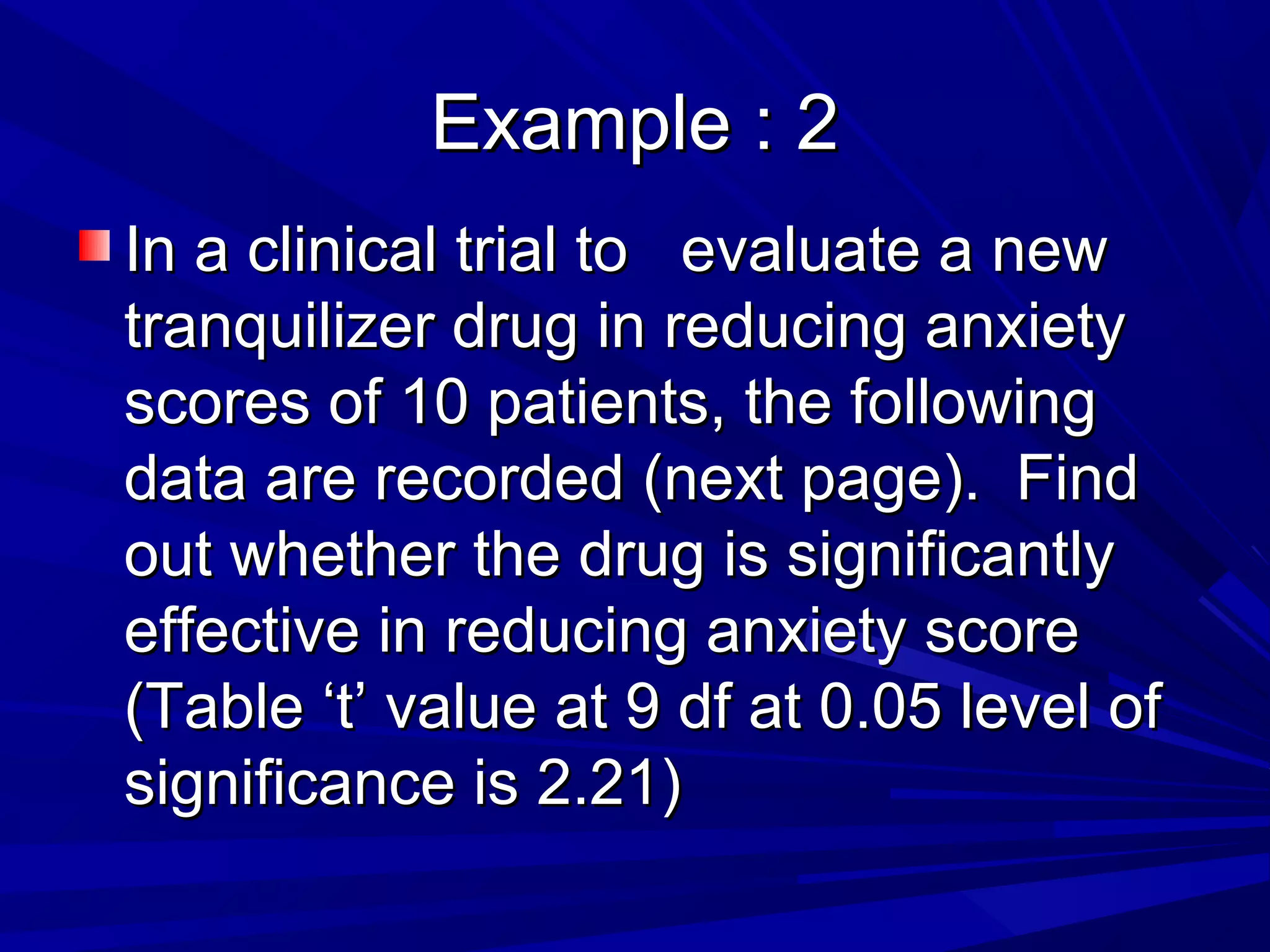
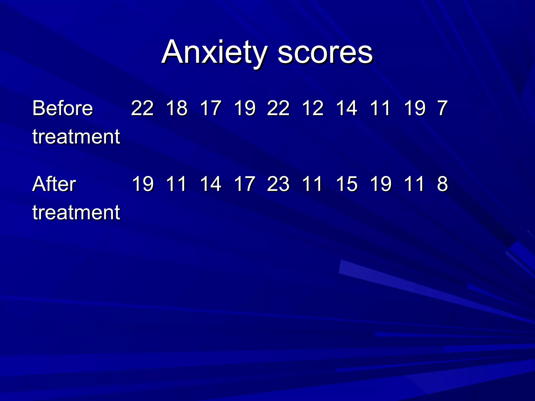
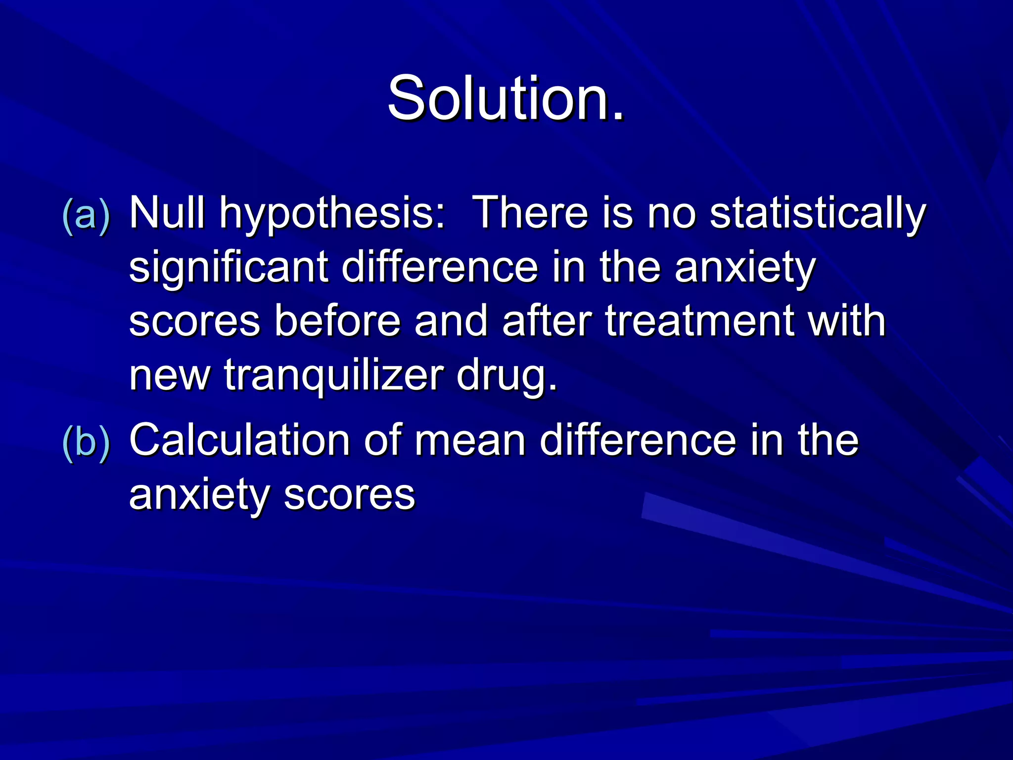
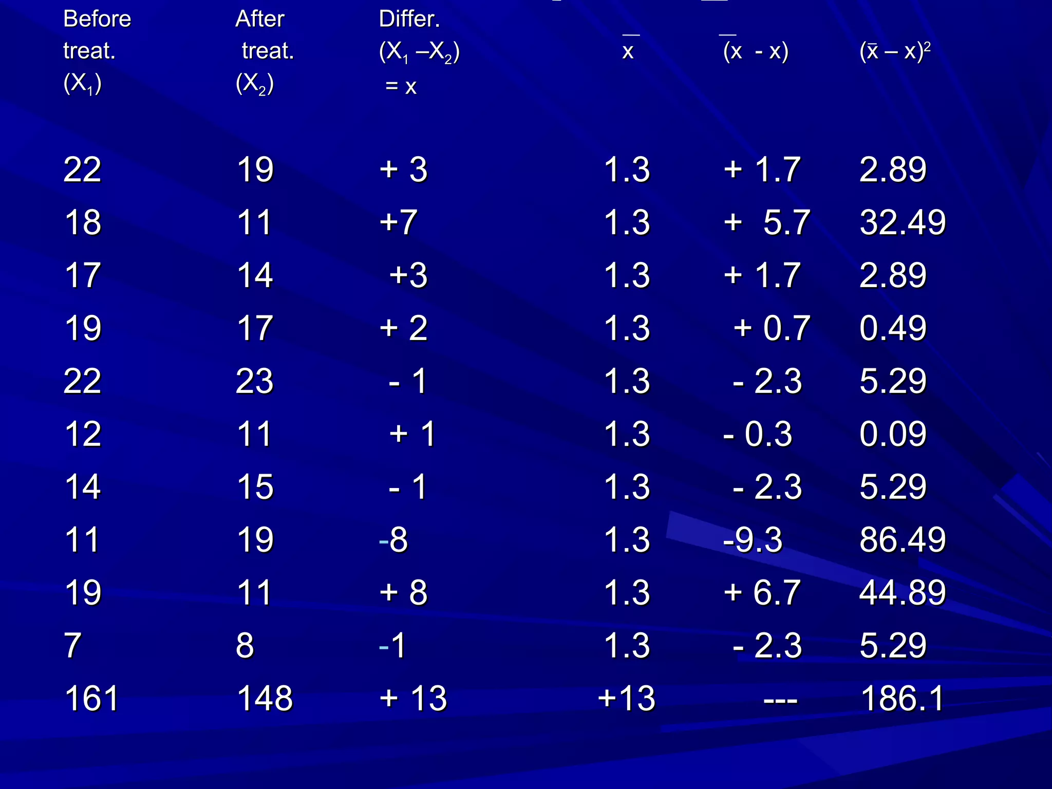
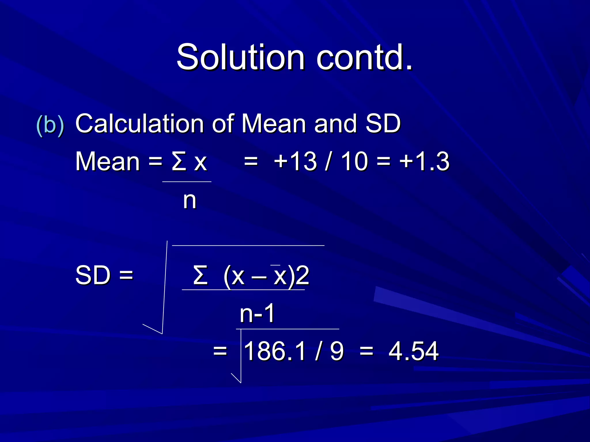
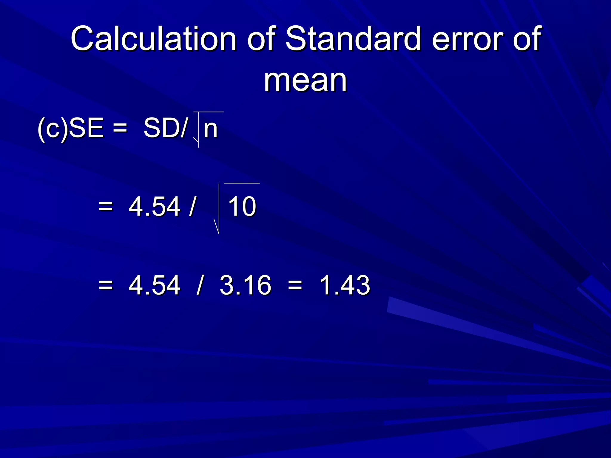
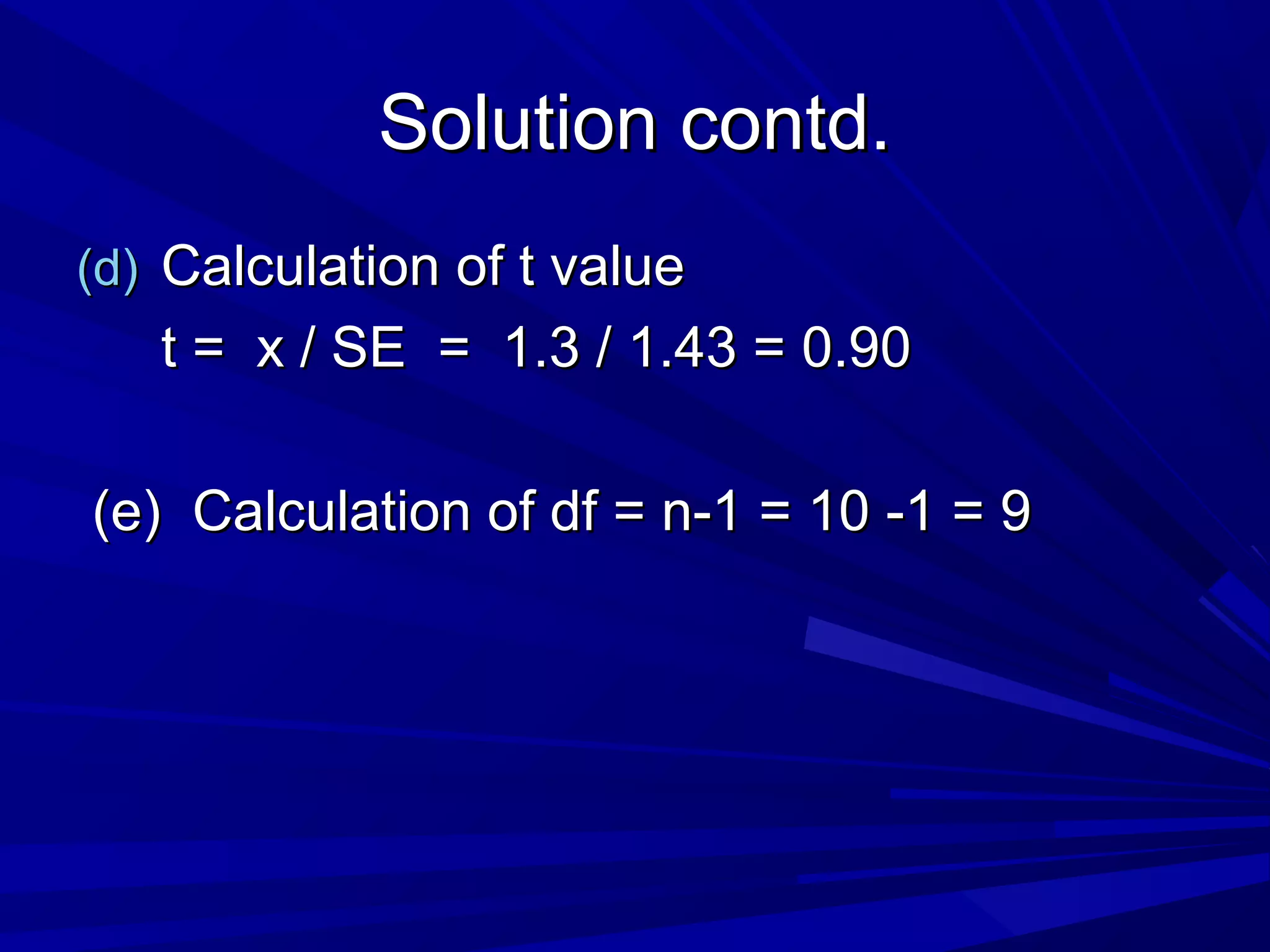
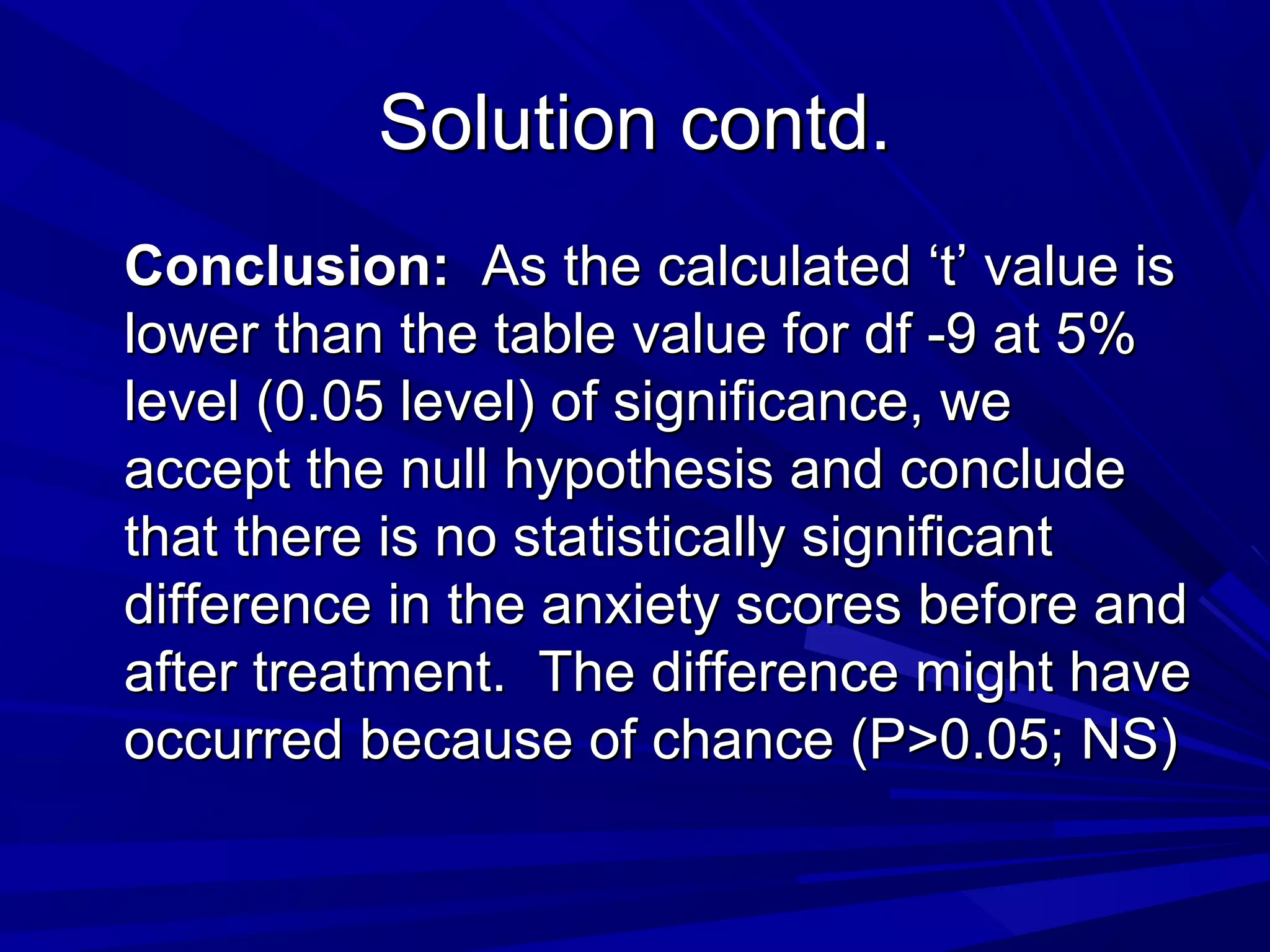
Student’s ‘t’ testStudent’s ‘t’ test
Dr. K . Ashok Kumar ReddyDr. K . Ashok Kumar Reddy
Professor & HODProfessor & HOD
, Dept. of Community Medicine, Dept. of Community Medicine
INTRODUCTIONINTRODUCTION
Very common test used in biomedicalVery common test used in biomedical
research.research.
Applied to test the significance ofApplied to test the significance of
difference between two means.difference between two means.
It has the advantage that it can be usedIt has the advantage that it can be used
for small samples (‘Z’ test can be used forfor small samples (‘Z’ test can be used for
large samples only)large samples only)
TypesTypes
Unpaired ‘t’ test or Pooled ‘t’ testUnpaired ‘t’ test or Pooled ‘t’ test
Paired ‘t’ test.Paired ‘t’ test.
Unpaired ‘t’ testUnpaired ‘t’ test
This is used to test the difference betweenThis is used to test the difference between
two independent samples.two independent samples.
Calculation is similar to ‘z’ test but withCalculation is similar to ‘z’ test but with
certain changes.certain changes.
Example: Question No. 1Example: Question No. 1
The chest circumference (in cm) of 10The chest circumference (in cm) of 10
normal and malnourished children of thenormal and malnourished children of the
same age group is given below:same age group is given below:
NormalNormal : 42, 46, 50, 48, 50, 52, 41, 49, 51, 56: 42, 46, 50, 48, 50, 52, 41, 49, 51, 56
MalnourishedMalnourished: 38, 41, 36, 35, 30, 42, 31, 29, 31, 35: 38, 41, 36, 35, 30, 42, 31, 29, 31, 35
Find out whether the mean chest circumference isFind out whether the mean chest circumference is
significantly different in the two groups (table ‘t’ value atsignificantly different in the two groups (table ‘t’ value at
18 df at 0.05 level of significance is 2.02)18 df at 0.05 level of significance is 2.02)
SolutionSolution
(a)(a) Null hypothesis: There is no statisticallyNull hypothesis: There is no statistically
significant difference in the mean chestsignificant difference in the mean chest
circumference between the two groups.circumference between the two groups.
(b)(b) Calculation of Standard error ofCalculation of Standard error of
difference between two means.difference between two means.
S (xS (x11 – x– x22) = S 1 + 1) = S 1 + 1
n1 n2n1 n2
where S is the combined SDwhere S is the combined SD
Solution contd.Solution contd.
Combined SD (S) =Combined SD (S) =
SS11
22
(n(n11-1) + S-1) + S22
22
(n(n22-1)-1)
nn11 + n+ n22 -2-2
where Swhere S11 and Sand S22 are Standard deviationsare Standard deviations
and nand n11 and nand n22 are the sample sizes of 1are the sample sizes of 1stst
and 2and 2ndnd
samples respectively.samples respectively.
Solution contd.Solution contd.
In the given example, following are theIn the given example, following are the
values of mean, SD and sample sizevalues of mean, SD and sample size
MeanMean SDSD NN
First sampleFirst sample 48.548.5 4.534.53 1010
Second sampleSecond sample 34.834.8 4.574.57 1010
By substituting the values, we getBy substituting the values, we get
4.534.5322
(10-1) + 4.57(10-1) + 4.5722
(10-1)(10-1)
10 + 10 - 210 + 10 - 2
Solution contd.Solution contd.
Thus, we getThus, we get
S = 20.52 (9) + 20.88 (9)S = 20.52 (9) + 20.88 (9)
1818
= 184. 68 + 187.96= 184. 68 + 187.96
1818
= 372.65 /18 = 20.70 = 4.55 cm= 372.65 /18 = 20.70 = 4.55 cm
Solution contd.Solution contd.
Thus SThus S (x1 – x2)(x1 – x2) = 4.55 1 + 1= 4.55 1 + 1
10 1010 10
= 4.55 0.1 + 0.1= 4.55 0.1 + 0.1
= 4.55 0.2= 4.55 0.2
= 4.55 X 0.44 = 2.03 cm= 4.55 X 0.44 = 2.03 cm
Solution contd.Solution contd.
(c)(c) Calculation of t valueCalculation of t value
t = Xt = X11 – X– X22
SS (x1 – x2)(x1 – x2)
= 48.5 – 34.8= 48.5 – 34.8
2.032.03
= 13.7/2.03 = 6.75= 13.7/2.03 = 6.75
Solution contd.Solution contd.
(d)(d) Degrees of freedom (df) = n1 + n2 -2Degrees of freedom (df) = n1 + n2 -2
= 10 + 10 – 2 = 20 -2 = 18.= 10 + 10 – 2 = 20 -2 = 18.
(e)(e) The maximum ‘t’ value for 18 df for 0.05The maximum ‘t’ value for 18 df for 0.05
level of significance is 2.02 (from table)level of significance is 2.02 (from table)
Solution contd.Solution contd.
(e)(e) Conclusion:Conclusion: As the calculated ‘t’ valueAs the calculated ‘t’ value
is higher than the table value for 18 dfis higher than the table value for 18 df
and 0.05 level of significance, we rejectand 0.05 level of significance, we reject
the null hypothesis and state that thethe null hypothesis and state that the
difference in the mean chestdifference in the mean chest
circumference values between normalcircumference values between normal
and malnourished groups is statisticallyand malnourished groups is statistically
significant. The difference might notsignificant. The difference might not
have occurred due to chancehave occurred due to chance
(P< 0.05; S)(P< 0.05; S)
Paired ‘t’ testPaired ‘t’ test
This test is used where each person givesThis test is used where each person gives
two observations – before and after valuestwo observations – before and after values
For example, if the same person gives twoFor example, if the same person gives two
observations before and after giving a newobservations before and after giving a new
drug – in such cases, this test is used.drug – in such cases, this test is used.
Example : 2Example : 2
In a clinical trial to evaluate a newIn a clinical trial to evaluate a new
tranquilizer drug in reducing anxietytranquilizer drug in reducing anxiety
scores of 10 patients, the followingscores of 10 patients, the following
data are recorded (next page). Finddata are recorded (next page). Find
out whether the drug is significantlyout whether the drug is significantly
effective in reducing anxiety scoreeffective in reducing anxiety score
(Table ‘t’ value at 9 df at 0.05 level of(Table ‘t’ value at 9 df at 0.05 level of
significance is 2.21)significance is 2.21)
Anxiety scoresAnxiety scores
BeforeBefore
treatmenttreatment
2222 1818 1717 1919 2222 1212 1414 1111 1919 77
AfterAfter
treatmenttreatment
1919 1111 1414 1717 2323 1111 1515 1919 1111 88
Solution.Solution.
(a)(a) Null hypothesis: There is no statisticallyNull hypothesis: There is no statistically
significant difference in the anxietysignificant difference in the anxiety
scores before and after treatment withscores before and after treatment with
new tranquilizer drug.new tranquilizer drug.
(b)(b) Calculation of mean difference in theCalculation of mean difference in the
anxiety scoresanxiety scores
BeforeBefore
treat.treat.
(X(X11))
AfterAfter
treat.treat.
(X(X22))
Differ.Differ.
(X(X11 –X–X22))
= x= x
xx (x - x)(x - x) (x – x)(x – x)22
2222 1919 + 3+ 3 1.31.3 + 1.7+ 1.7 2.892.89
1818 1111 +7+7 1.31.3 + 5.7+ 5.7 32.4932.49
1717 1414 +3+3 1.31.3 + 1.7+ 1.7 2.892.89
1919 1717 + 2+ 2 1.31.3 + 0.7+ 0.7 0.490.49
2222 2323 - 1- 1 1.31.3 - 2.3- 2.3 5.295.29
1212 1111 + 1+ 1 1.31.3 - 0.3- 0.3 0.090.09
1414 1515 - 1- 1 1.31.3 - 2.3- 2.3 5.295.29
1111 1919 -88 1.31.3 -9.3-9.3 86.4986.49
1919 1111 + 8+ 8 1.31.3 + 6.7+ 6.7 44.8944.89
77 88 -11 1.31.3 - 2.3- 2.3 5.295.29
161161 148148 + 13+ 13 +13+13 ------ 186.1186.1
Solution contd.Solution contd.
(b)(b) Calculation of Mean and SDCalculation of Mean and SD
Mean =Mean = ΣΣ x = +13 / 10 = +1.3x = +13 / 10 = +1.3
nn
SD =SD = ΣΣ (x – x)2(x – x)2
n-1n-1
= 186.1 / 9 = 4.54= 186.1 / 9 = 4.54
Calculation of Standard error ofCalculation of Standard error of
meanmean
(c)SE = SD/ n(c)SE = SD/ n
= 4.54 / 10= 4.54 / 10
= 4.54 / 3.16 = 1.43= 4.54 / 3.16 = 1.43
Solution contd.Solution contd.
(d)(d) Calculation of t valueCalculation of t value
t = x / SE = 1.3 / 1.43 = 0.90t = x / SE = 1.3 / 1.43 = 0.90
(e) Calculation of df = n-1 = 10 -1 = 9(e) Calculation of df = n-1 = 10 -1 = 9
Solution contd.Solution contd.
Conclusion:Conclusion: As the calculated ‘t’ value isAs the calculated ‘t’ value is
lower than the table value for df -9 at 5%lower than the table value for df -9 at 5%
level (0.05 level) of significance, welevel (0.05 level) of significance, we
accept the null hypothesis and concludeaccept the null hypothesis and conclude
that there is no statistically significantthat there is no statistically significant
difference in the anxiety scores before anddifference in the anxiety scores before and
after treatment. The difference might haveafter treatment. The difference might have
occurred because of chance (P>0.05; NS)occurred because of chance (P>0.05; NS)

Student t t est

  • 1.
    Student’s ‘t’ testStudent’s‘t’ test Dr. K . Ashok Kumar ReddyDr. K . Ashok Kumar Reddy Professor & HODProfessor & HOD , Dept. of Community Medicine, Dept. of Community Medicine
  • 2.
    INTRODUCTIONINTRODUCTION Very common testused in biomedicalVery common test used in biomedical research.research. Applied to test the significance ofApplied to test the significance of difference between two means.difference between two means. It has the advantage that it can be usedIt has the advantage that it can be used for small samples (‘Z’ test can be used forfor small samples (‘Z’ test can be used for large samples only)large samples only)
  • 3.
    TypesTypes Unpaired ‘t’ testor Pooled ‘t’ testUnpaired ‘t’ test or Pooled ‘t’ test Paired ‘t’ test.Paired ‘t’ test.
  • 4.
    Unpaired ‘t’ testUnpaired‘t’ test This is used to test the difference betweenThis is used to test the difference between two independent samples.two independent samples. Calculation is similar to ‘z’ test but withCalculation is similar to ‘z’ test but with certain changes.certain changes.
  • 5.
    Example: Question No.1Example: Question No. 1 The chest circumference (in cm) of 10The chest circumference (in cm) of 10 normal and malnourished children of thenormal and malnourished children of the same age group is given below:same age group is given below: NormalNormal : 42, 46, 50, 48, 50, 52, 41, 49, 51, 56: 42, 46, 50, 48, 50, 52, 41, 49, 51, 56 MalnourishedMalnourished: 38, 41, 36, 35, 30, 42, 31, 29, 31, 35: 38, 41, 36, 35, 30, 42, 31, 29, 31, 35 Find out whether the mean chest circumference isFind out whether the mean chest circumference is significantly different in the two groups (table ‘t’ value atsignificantly different in the two groups (table ‘t’ value at 18 df at 0.05 level of significance is 2.02)18 df at 0.05 level of significance is 2.02)
  • 6.
    SolutionSolution (a)(a) Null hypothesis:There is no statisticallyNull hypothesis: There is no statistically significant difference in the mean chestsignificant difference in the mean chest circumference between the two groups.circumference between the two groups. (b)(b) Calculation of Standard error ofCalculation of Standard error of difference between two means.difference between two means. S (xS (x11 – x– x22) = S 1 + 1) = S 1 + 1 n1 n2n1 n2 where S is the combined SDwhere S is the combined SD
  • 7.
    Solution contd.Solution contd. CombinedSD (S) =Combined SD (S) = SS11 22 (n(n11-1) + S-1) + S22 22 (n(n22-1)-1) nn11 + n+ n22 -2-2 where Swhere S11 and Sand S22 are Standard deviationsare Standard deviations and nand n11 and nand n22 are the sample sizes of 1are the sample sizes of 1stst and 2and 2ndnd samples respectively.samples respectively.
  • 8.
    Solution contd.Solution contd. Inthe given example, following are theIn the given example, following are the values of mean, SD and sample sizevalues of mean, SD and sample size MeanMean SDSD NN First sampleFirst sample 48.548.5 4.534.53 1010 Second sampleSecond sample 34.834.8 4.574.57 1010 By substituting the values, we getBy substituting the values, we get 4.534.5322 (10-1) + 4.57(10-1) + 4.5722 (10-1)(10-1) 10 + 10 - 210 + 10 - 2
  • 9.
    Solution contd.Solution contd. Thus,we getThus, we get S = 20.52 (9) + 20.88 (9)S = 20.52 (9) + 20.88 (9) 1818 = 184. 68 + 187.96= 184. 68 + 187.96 1818 = 372.65 /18 = 20.70 = 4.55 cm= 372.65 /18 = 20.70 = 4.55 cm
  • 10.
    Solution contd.Solution contd. ThusSThus S (x1 – x2)(x1 – x2) = 4.55 1 + 1= 4.55 1 + 1 10 1010 10 = 4.55 0.1 + 0.1= 4.55 0.1 + 0.1 = 4.55 0.2= 4.55 0.2 = 4.55 X 0.44 = 2.03 cm= 4.55 X 0.44 = 2.03 cm
  • 11.
    Solution contd.Solution contd. (c)(c)Calculation of t valueCalculation of t value t = Xt = X11 – X– X22 SS (x1 – x2)(x1 – x2) = 48.5 – 34.8= 48.5 – 34.8 2.032.03 = 13.7/2.03 = 6.75= 13.7/2.03 = 6.75
  • 12.
    Solution contd.Solution contd. (d)(d)Degrees of freedom (df) = n1 + n2 -2Degrees of freedom (df) = n1 + n2 -2 = 10 + 10 – 2 = 20 -2 = 18.= 10 + 10 – 2 = 20 -2 = 18. (e)(e) The maximum ‘t’ value for 18 df for 0.05The maximum ‘t’ value for 18 df for 0.05 level of significance is 2.02 (from table)level of significance is 2.02 (from table)
  • 13.
    Solution contd.Solution contd. (e)(e)Conclusion:Conclusion: As the calculated ‘t’ valueAs the calculated ‘t’ value is higher than the table value for 18 dfis higher than the table value for 18 df and 0.05 level of significance, we rejectand 0.05 level of significance, we reject the null hypothesis and state that thethe null hypothesis and state that the difference in the mean chestdifference in the mean chest circumference values between normalcircumference values between normal and malnourished groups is statisticallyand malnourished groups is statistically significant. The difference might notsignificant. The difference might not have occurred due to chancehave occurred due to chance (P< 0.05; S)(P< 0.05; S)
  • 14.
    Paired ‘t’ testPaired‘t’ test This test is used where each person givesThis test is used where each person gives two observations – before and after valuestwo observations – before and after values For example, if the same person gives twoFor example, if the same person gives two observations before and after giving a newobservations before and after giving a new drug – in such cases, this test is used.drug – in such cases, this test is used.
  • 15.
    Example : 2Example: 2 In a clinical trial to evaluate a newIn a clinical trial to evaluate a new tranquilizer drug in reducing anxietytranquilizer drug in reducing anxiety scores of 10 patients, the followingscores of 10 patients, the following data are recorded (next page). Finddata are recorded (next page). Find out whether the drug is significantlyout whether the drug is significantly effective in reducing anxiety scoreeffective in reducing anxiety score (Table ‘t’ value at 9 df at 0.05 level of(Table ‘t’ value at 9 df at 0.05 level of significance is 2.21)significance is 2.21)
  • 16.
    Anxiety scoresAnxiety scores BeforeBefore treatmenttreatment 22221818 1717 1919 2222 1212 1414 1111 1919 77 AfterAfter treatmenttreatment 1919 1111 1414 1717 2323 1111 1515 1919 1111 88
  • 17.
    Solution.Solution. (a)(a) Null hypothesis:There is no statisticallyNull hypothesis: There is no statistically significant difference in the anxietysignificant difference in the anxiety scores before and after treatment withscores before and after treatment with new tranquilizer drug.new tranquilizer drug. (b)(b) Calculation of mean difference in theCalculation of mean difference in the anxiety scoresanxiety scores
  • 18.
    BeforeBefore treat.treat. (X(X11)) AfterAfter treat.treat. (X(X22)) Differ.Differ. (X(X11 –X–X22)) = x=x xx (x - x)(x - x) (x – x)(x – x)22 2222 1919 + 3+ 3 1.31.3 + 1.7+ 1.7 2.892.89 1818 1111 +7+7 1.31.3 + 5.7+ 5.7 32.4932.49 1717 1414 +3+3 1.31.3 + 1.7+ 1.7 2.892.89 1919 1717 + 2+ 2 1.31.3 + 0.7+ 0.7 0.490.49 2222 2323 - 1- 1 1.31.3 - 2.3- 2.3 5.295.29 1212 1111 + 1+ 1 1.31.3 - 0.3- 0.3 0.090.09 1414 1515 - 1- 1 1.31.3 - 2.3- 2.3 5.295.29 1111 1919 -88 1.31.3 -9.3-9.3 86.4986.49 1919 1111 + 8+ 8 1.31.3 + 6.7+ 6.7 44.8944.89 77 88 -11 1.31.3 - 2.3- 2.3 5.295.29 161161 148148 + 13+ 13 +13+13 ------ 186.1186.1
  • 19.
    Solution contd.Solution contd. (b)(b)Calculation of Mean and SDCalculation of Mean and SD Mean =Mean = ΣΣ x = +13 / 10 = +1.3x = +13 / 10 = +1.3 nn SD =SD = ΣΣ (x – x)2(x – x)2 n-1n-1 = 186.1 / 9 = 4.54= 186.1 / 9 = 4.54
  • 20.
    Calculation of Standarderror ofCalculation of Standard error of meanmean (c)SE = SD/ n(c)SE = SD/ n = 4.54 / 10= 4.54 / 10 = 4.54 / 3.16 = 1.43= 4.54 / 3.16 = 1.43
  • 21.
    Solution contd.Solution contd. (d)(d)Calculation of t valueCalculation of t value t = x / SE = 1.3 / 1.43 = 0.90t = x / SE = 1.3 / 1.43 = 0.90 (e) Calculation of df = n-1 = 10 -1 = 9(e) Calculation of df = n-1 = 10 -1 = 9
  • 22.
    Solution contd.Solution contd. Conclusion:Conclusion:As the calculated ‘t’ value isAs the calculated ‘t’ value is lower than the table value for df -9 at 5%lower than the table value for df -9 at 5% level (0.05 level) of significance, welevel (0.05 level) of significance, we accept the null hypothesis and concludeaccept the null hypothesis and conclude that there is no statistically significantthat there is no statistically significant difference in the anxiety scores before anddifference in the anxiety scores before and after treatment. The difference might haveafter treatment. The difference might have occurred because of chance (P>0.05; NS)occurred because of chance (P>0.05; NS)