
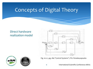
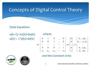


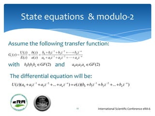


1) The document discusses state equations that can model digital control systems based on modulo-2 arithmetic and their application to recursive convolutional coding. 2) State equations can be derived from the transfer function of a discrete-time controller and expressed using modulo-2 arithmetic. 3) A recursive convolutional encoder can be modeled by state equations in modulo-2 algebra, where the state at each time step is a function of the previous states and the input bit.


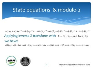
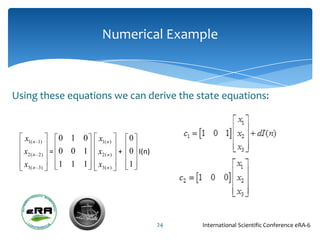
![[Vvedensky d.] group_theory,_problems_and_solution(book_fi.org)](https://cdn.slidesharecdn.com/ss_thumbnails/vvedenskyd-grouptheoryproblemsandsolutionbookfi-org-130405071812-phpapp02-thumbnail.jpg?width=640&height=640&fit=bounds)


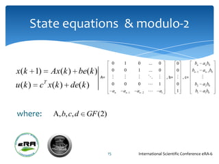
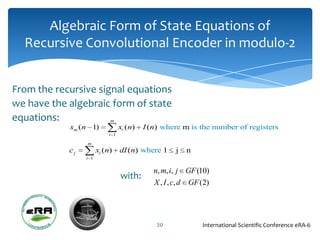
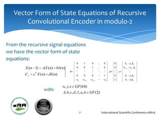
![5G Explained! A High Level Overview [Introduction]](https://cdn.slidesharecdn.com/ss_thumbnails/5gexplainedahighleveloverview-260119165306-cc137a3e-thumbnail.jpg?width=640&height=640&fit=bounds)


