This document discusses various structures for implementing finite impulse response (FIR) and infinite impulse response (IIR) digital filters. It begins by introducing linear constant coefficient difference equations (LCCDEs) and signal flowgraphs used to represent digital filters. It then covers direct form, cascade form, and other implementations for FIR filters, including exploiting symmetry for linear phase filters. For IIR filters, it discusses direct form I and II, cascade, and parallel implementations using factorizations of the filter transfer function. Examples are provided to illustrate different filter realizations.

1. EE385: Introduction to Digital Signal Processing
Chapter 6: Design of FIR and IIR Filters
Dr. Mohammed W. Baidas
Professor
Department of Electrical Engineering
College of Engineering and Petroleum
Kuwait University
EE385: Introduction to Digital Signal Processing - Chapter 6 Prof. M. W. Baidas 1/19

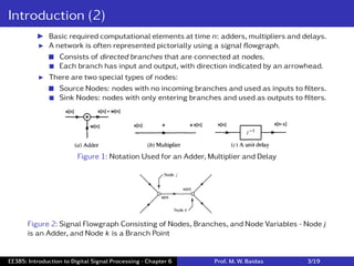
2. Introduction (1)
• Given an LTI system with a rational system function H[z], the input and output are
related by an LCCDE.
I For example, with a system function
H[z] =
b[0] + b[1]z−1
1 + a[1]z−1
, (1)
the input x[n] and output y[n] are related by the LCCDE
y[n] = −a[1]y[n − 1] + b[0]x[n] + b[1]x[n − 1]. (2)
I Note that this system may also be implemented with the following pair of coupled
difference equations
w[n] = −a[1]w[n − 1] + x[n]
y[n] = b[0]w[n] + b[1]w[n − 1].
(3)
With this implementation, it is only necessary to provide one memory
location to store w[n − 1]; whereas Eq. (2) requires two memory locations,
one to store y[n − 1] and one to store x[n − 1].
I This suggests that the amount of computation and/or memory required will de-
pend on the implementation.
• For a linear time-invariant system with a rational system function, the input x[n] and
the output y[n] are related by an LCCDE
y[n] =
q
∑
k=0
b[k]x[n − k] −
p
∑
k=1
a[k]y[n − k]. (4)
EE385: Introduction to Digital Signal Processing - Chapter 6 Prof. M. W. Baidas 2/19

3. Introduction (2)
I Basic required computational elements at time n: adders, multipliers and delays.
I A network is often represented pictorially using a signal flowgraph.
Consists of directed branches that are connected at nodes.
Each branch has input and output, with direction indicated by an arrowhead.
I There are two special types of nodes:
Source Nodes: nodes with no incoming branches and used as inputs to filters.
Sink Nodes: nodes with only entering branches and used as outputs to filters.
Figure 1: Notation Used for an Adder, Multiplier and Delay
Figure 2: Signal Flowgraph Consisting of Nodes, Branches, and Node Variables - Node j
is an Adder, and Node k is a Branch Point
EE385: Introduction to Digital Signal Processing - Chapter 6 Prof. M. W. Baidas 3/19

4. Structures for FIR Systems (1)
• A causal finite impulse response (FIR) filter has a system function that is polynomial in
z−1, as
H[z] =
N
∑
n=0
h[n]z−n. (5)
I For an input x[n], the output is
y[n] =
N
∑
k=0
h[k]x[n − k].
For each value of n, evaluating this sum requires N + 1 multiplications and N
additions.
• Direct Form:
I Implement an FIR filter is in direct form using a tapped delay line.
This structure requires N + 1 multiplications, N additions, N delays.
Figure 3: Direct Form Implementation of FIR Filters
EE385: Introduction to Digital Signal Processing - Chapter 6 Prof. M. W. Baidas 4/19

5. Structures for FIR Systems (2)
• Cascade Form:
I For a causal FIR filter, the system function may be factored into a product of first-
order factors,
H[z] =
N
∑
n=0
h[n]z−n = A
N
∏
k=1
(
1 − αk z−1
)
, (6)
where αk for k = 1,2,...,N are the zeros of H[z].
If h[n] is real, the complex roots of H[z] occur in complex conjugate pairs.
These conjugate pairs may be combined to form second-order factors with
real coefficients,
H[z] = A
Ns
∏
k=1
[
1 + bk [1]z−1 + bk [2]z−2
]
. (7)
Written in this form, H[z] may be implemented as a cascade of second-order
FIR filters.
Figure 4: An FIR Filter Implemented as a Cascade of Second-Order Systems
EE385: Introduction to Digital Signal Processing - Chapter 6 Prof. M. W. Baidas 5/19

6. Structures for FIR Systems (3)
• Linear Phase Filters:
I Linear phase filters have a unit sample response that is either symmetric,
h[n] = h[N − n], (8)
or antisymmetric,
h[n] = −h[N − n]. (9)
I This symmetry may be exploited to simplify the network structure.
I For example, if N is even and h[n] is symmetric (type I filter),
y[n] =
N
∑
n=0
h[k]x[n − k] =
N/2−1
∑
k=0
h[k][x[n − k] + x[n − N + k]] + h
[
N
2
]
x
[
n −
N
2
]
.
(10)
Therefore, forming the sums [x[n − k] + x[n − N + k]] prior to multiplying by
h[k] reduces the number of multiplications.
Figure 5: Direct Form Implementation of Type I Linear Phase Filter
EE385: Introduction to Digital Signal Processing - Chapter 6 Prof. M. W. Baidas 6/19

7. Structures for FIR Systems (4)
I If N is odd and h[n] is symmetric, then a type II linear phase filter is obtained.
Figure 6: Direct Form Implementation of Type II Linear Phase Filter
I Example 6.1: An LTI system has a unit sample response given by h[n] =
{−0.01,0.02,−0.10,0.40,−0.10,0.02,−0.01}. Draw a signal flowgraph for this sys-
tem that requires the minimum number of multiplications.
EE385: Introduction to Digital Signal Processing - Chapter 6 Prof. M. W. Baidas 7/19

8. Structures for IIR Systems (1)
• The input x[n] and output y[n] of a causal IIR filter with a rational system function
H[z] =
B[z]
A[z]
=
∑q
k=0 b[k]z−k
1 +
∑p
k=1 a[k]z−k
(11)
is described by the LCCDE
y[n] =
q
∑
k=0
b[k]x[n − k] −
p
∑
k=1
a[k]y[n − k]. (12)
• Direct Form:
I Two direct form filter structures: direct form I and direct form II.
I Direct Form I:
An implementation that results when Eq. (12) is written as
w[n] =
q
∑
k=0
b[k]x[n − k]
y[n] = w[n] −
p
∑
k=1
a[k]y[n − k].
(13)
First equation corresponds to an FIR filter with input x[n], and output w[n];
while second equation corresponds to an all-pole filter with input w[n] and
output y[n].
EE385: Introduction to Digital Signal Processing - Chapter 6 Prof. M. W. Baidas 8/19

9. Structures for IIR Systems (2)
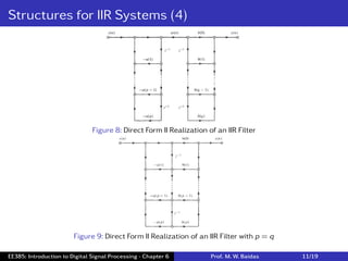
Figure 7: Direct Form I Realization of an IIR Filter
• Direct Form: (Continued)
I Direct Form I: (Continued)
Therefore, this pair of equations represents a cascade of two systems,
Y[z] =
1
A[z]
[B[z]X[z]]. (14)
Computational requirements for a Direct Form I structure are as follows:
Number of multiplications: p + q + 1 per output sample.
Number of additions: p + q per output sample.
Number of delays: p + q.
EE385: Introduction to Digital Signal Processing - Chapter 6 Prof. M. W. Baidas 9/19

10. Structures for IIR Systems (3)
• Direct Form: (Continued)
I Direct Form II:
Structure is obtained by reversing order of cascade of B[z] and 1/A[z], such
that x[n] is first filtered with the all-pole filter 1/A[z] and then with B[z], as
Y[z] = B[z]
[
1
A[z]
X[z]
]
. (15)
If we denote the output of the all-pole filter 1/A[z] by w[n], this structure is
given by
w[n] = x[n] −
p
∑
k=1
a[k]w[n − k]
y[n] =
q
∑
k=0
b[k]w[n − k].
(16)
This structure may be simplified by noting that the two sets of delays are
delaying the same sequence. Therefore, they may be combined.
Computational requirements for a Direct Form II structure are as follows:
Number of multiplications: p + q + 1 per output sample.
Number of additions: p + q per output sample.
Number of delays: max(p,q).
Direct form II structure is said to be canonic because it uses the minimum
number of delays for a given H[z].
EE385: Introduction to Digital Signal Processing - Chapter 6 Prof. M. W. Baidas 10/19

11. Structures for IIR Systems (4)
Figure 8: Direct Form II Realization of an IIR Filter
Figure 9: Direct Form II Realization of an IIR Filter with p = q
EE385: Introduction to Digital Signal Processing - Chapter 6 Prof. M. W. Baidas 11/19

12. Structures for IIR Systems (5)
• Cascade Structure:
I The cascade structure is derived by factoring the numerator and denominator
polynomials of H[z]:
H[z] =
∑q
k=0 b[k]z−k
1 +
∑p
k=1 a[k]z−k
= A
max(p,q)
∏
k=1
1 − βk z−1
1 − αk z−1
. (17)
This factorization corresponds to a cascade of first-order filters, each having
one pole and one zero.
In general, the coefficients αk and βk will be complex.
However, if h[n] is real, roots of H[z] will occur in complex conjugate pairs,
and these complex conjugate factors may be combined to form second-order
factors with real coefficients, such that
Hk [z] =
1 + β1k z−1 + β2k z−2
1 + α1k z−1 + α2k z−2
. (18)
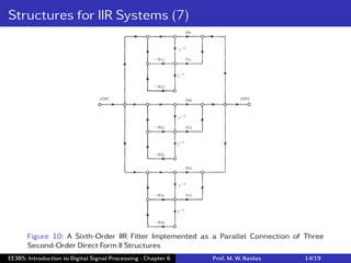
I A sixth-order IIR filter implemented as a cascade of three second-order systems
in direct form II is shown below.
EE385: Introduction to Digital Signal Processing - Chapter 6 Prof. M. W. Baidas 12/19

13. Structures for IIR Systems (6)
• Parallel Structure:
I An alternative to factoring H[z] is to expand the system function using a partial
fraction expansion. For example, with
H[z] =
∑q
k=0 b[k]z−k
1 +
∑p
k=1 a[k]z−k
= A
∏q
k=1
(
1 − βk z−1
)
∏p
k=1
(
1 − αk z−1
) , (19)
if p q and αi , αj (i.e. roots of denominator polynomial are distinct), H[z] may
be expanded as a sum of p first-order factors as follows:
H[z] =
p
∑
k=1
Ak
1 − αk z−1
, (20)
where the coefficients Ak , and αk are, in general, complex.
This expansion corresponds to a sum of p first-order system functions and
may be realized by connecting these systems in parallel.
If h[n] is real, the poles of H[z] will occur in complex conjugate pairs, and
these complex roots in the partial fraction expansion may be combined to
form second-order systems with real coefficients, as
H[z] =
Ns
∑
k=1
γ0k + γ1k z−1
1 + α1k z−1 + α2k z−2
. (21)
I If p ≤ q, the partial fraction expansion will also contain a term of the form
c0 + c1z−1 + ··· + cq−pz−(q−p), (22)
which is an FIR filter in parallel with the other terms in the expansion of H[z].
EE385: Introduction to Digital Signal Processing - Chapter 6 Prof. M. W. Baidas 13/19

14. Structures for IIR Systems (7)
Figure 10: A Sixth-Order IIR Filter Implemented as a Parallel Connection of Three
Second-Order Direct Form II Structures
EE385: Introduction to Digital Signal Processing - Chapter 6 Prof. M. W. Baidas 14/19

15. Structures for IIR Systems (8)
• Example 6.2: Consider the causal LTI filter with system function
H[z] =
1 + 0.875z−1
(
1 + 0.2z−1 + 0.9z−2
)(
1 − 0.7z−1
) .
Draw a signal flowgraph for this system using:
(a) Direct form I.
(b) Direct form II.
(c) Cascade of first- and second-order systems realized in direct form II.
(d) Parallel connection of first- and second-order systems realized in direct form II.
Solution:
(a) Writing the system function as a ratio of polynomials in z−1, yields
H[z] =
1 + 0.875z−1
1 − 0.5z−1 + 0.76z−2 − 0.63z−3
,
it follows that the direct form I realization of H[z] is as follows.
EE385: Introduction to Digital Signal Processing - Chapter 6 Prof. M. W. Baidas 15/19

16. Structures for IIR Systems (9)
• Example 6.2: (Continued)
(b) For a direct form II realization of H[z], we have
(c) The realization of H[z] is as follows:
EE385: Introduction to Digital Signal Processing - Chapter 6 Prof. M. W. Baidas 16/19

17. Structures for IIR Systems (10)
• Example 6.2: (Continued)
(d) For a parallel structure, H[z] must be expanded using a partial fraction expan-
sion,
H[z] =
1 + 0.875z−1
(
1 + 0.2z−1 + 0.9z−2
)(
1 − 0.7z−1
) =
A + Bz−1
1 + 0.2z−1 + 0.9z−2
+
C
1 − 0.7z−1
.
(23)
Solving for A, B, and C, we find A = 0.2794, B = 0.9265, and C = 0.7206. There-
fore, the partial fraction expansion is
H[z] =
0.2794 + 0.9265z−1
1 + 0.2z−1 + 0.9z−2
+
0.7206
1 − 0.7z−1
. (24)
Thus, a parallel structure for H[z] is shown below.
EE385: Introduction to Digital Signal Processing - Chapter 6 Prof. M. W. Baidas 17/19

18. Solved Problems (1)
• S-Problem 7.1: Draw the structure of the FIR filter for
y[n] =
3
∑
k=0
b[k]x[n − k] = 3x[n] + 3x[n − 1] + 2x[n − 2] − 2x[n − 3].
Figure 11: FIR Filter Structure of S-Problem 7.1
• S-Problem 7.2: Consider the filter structure shown in the figure below. Find the system
function and the unit sample response of this system.
EE385: Introduction to Digital Signal Processing - Chapter 6 Prof. M. W. Baidas 18/19

19. Solved Problems (2)
• S-Problem 7.2:
Solution: For the three nodes labeled in the flowgraph below, we have the following
node equations:
w[n] = x[n] + 0.2w[n − 1]
v[n] = x[n] + w[n]
y[n] = v[n] + 2w[n − 1].
Using the z−transforms, the first equation becomes W[z] = 1
1−0.2z−1 X[z]. Taking the
z−transform of the second equation, and substituting the expression above for W[z],
we have
V[z] = X[z] + W[z] = X[z] +
1
1 − 0.2z−1
X[z] =
2 − 0.2z−1
1 − 0.2z−1
X[z].
Finally, taking the z−transform of the last equation, we find
Y[z] = V[z] + 2z−1W[z] =
[
2 − 0.2z−1
1 − 0.2z−1
+ 2z−1 1
1 − 0.2z−1
]
X[z] =
2 + 1.8z−1
1 − 0.2z−1
X[z].
Therefore, the system function is H[z] = 2+1.8z−1
1−0.2z−1 , and the unit sample response is
h[n] = 2(0.2)nu[n] + 1.8(0.2)n−1u[n − 1].
EE385: Introduction to Digital Signal Processing - Chapter 6 Prof. M. W. Baidas 19/19