Introduction HDDT Unbalanced and drifting data streams Experimental results Conclusion
Using HDDT to avoid instances propagation
in unbalanced and evolving data streams
IJCNN 2014
Andrea Dal Pozzolo, Reid Johnson, Olivier Caelen,
Serge Waterschoot, Nitesh V Chawla and Gianluca
Bontempi
07/07/2014
1/ 27
Introduction HDDT Unbalanced and drifting data streams Experimental results Conclusion
INTRODUCTION
In many applications (e.g. Fraud detection), we have a
stream of observations that we want to classify in real time.
When one class is rare, the classification problem is said to
be unbalanced.
In this paper we focus unbalanced data stream with two
classes, positive (minority) and negative (majority).
In unbalanced data streams, state-of-the-art techniques use
instance propagation and standard decision trees (e.g.
C4.5 [13]).
However, it is not always possible to either revisit or store
old instances of a data stream.
2/ 27
Introduction HDDT Unbalanced and drifting data streams Experimental results Conclusion
INTRODUCTION II
We use Hellinger Distance Decision Tree [7] (HDDT) to
deal with skewed distributions in data streams.
We consider data streams where the instances are received
over time in streams of batches.
HDDT allows us to remove instance propagations between
batches, benefits:
improved predictive accuracy
speed
single-pass through the data.
An ensemble of HDDTs is used to combat concept drift
and increase the accuracy of single classifiers.
We test our framework on several streaming datasets with
unbalanced classes and concept drift.
3/ 27
Introduction HDDT Unbalanced and drifting data streams Experimental results Conclusion
HELLINGER DISTANCE DECISION TREES
HDDT [6] use Hellinger Distance as splitting criteria in
decision trees for unbalanced problems.
All numerical features are partitioned into p bins (only
categorical variables).
The Hellinger Distance between the positive and negative
class is computed for each feature and then the feature
with the maximum distance is used to split the tree.
dH(f+, f−) =
p
j=1
|f+j|
|f+|
−
|f−j|
|f−|
2
(1)
where f+ denote the positive instances and f− the negatives of
feature f. Note that the class priors do not appear explicitly in
equation 1.
4/ 27
Introduction HDDT Unbalanced and drifting data streams Experimental results Conclusion
CONCEPT DRIFT
The concept to learn can change due to non-stationary
distributions.
In the presence of concept drift, we cannot longer assume
that the training and testing batches come from the same
distribution.
Concept drift [11] can occur due to a change in:
P(c), class priors.
P(x|c), distribution of the classes.
P(c|x), posterior distributions of class membership.
5/ 27
Introduction HDDT Unbalanced and drifting data streams Experimental results Conclusion
CONCEPT DRIFT II
In general we don’t know where the changes in distributions
come from, but we can measure the distances between two
batches to estimate the similarities of the distributions.
If the batch used for training a model is not similar to the
testing batch, we can assume that the model is obsolete.
In our work we use batch distances to assign low weights
to obsolete models.
6/ 27
Introduction HDDT Unbalanced and drifting data streams Experimental results Conclusion
HELLINGER DISTANCE BETWEEN BATCHES
Let Bt be the batch at time t used for training and Bt+1 the
subsequent testing batch. We compute the distance between Bt
and Bt+1 for a given feature f using Hellinger distance as
proposed by Lichtenwalter and Chawla [12]:
HD(Bt
, Bt+1
, f) =
v∈f


|Bt
f=v|
|Bt|
−
|Bt+1
f=v|
|Bt+1|


2
(2)
where |Bt
f=v| is the number of instances of feature f taking value
v in the batch at time t, while |Bt| is the total number of
instances in the same batch.
7/ 27
Introduction HDDT Unbalanced and drifting data streams Experimental results Conclusion
INFORMATION GAIN
Equation 2 does not account for differences in feature
relevance.
Lichtenwalter and Chawla [12] suggest to use the
information gain to weight the distances.
For a given feature f of a batch B, the Information Gain (IG) is
defined as the decrease in entropy E of a class c:
IG(B, f) = E(Bc) − E(Bc|Bf ) (3)
where Bc defines the class of the observations in batch B and Bf
the observations of feature f.
8/ 27
Introduction HDDT Unbalanced and drifting data streams Experimental results Conclusion
HELLINGER DISTANCE AND INFORMATION GAIN
We can make the assumption that feature relevance remains
stable over time and define a new distance function that
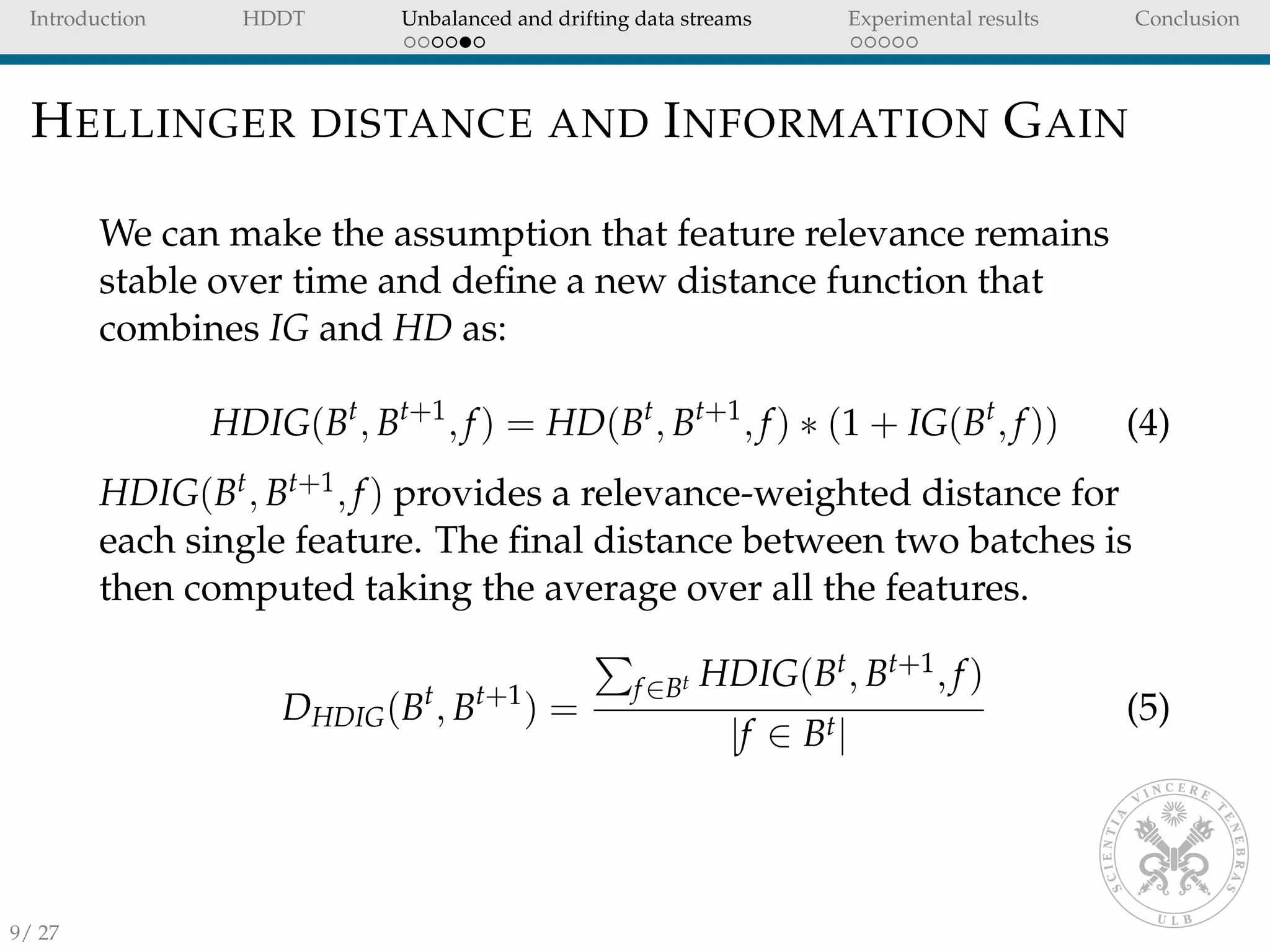
combines IG and HD as:
HDIG(Bt
, Bt+1
, f) = HD(Bt
, Bt+1
, f) ∗ (1 + IG(Bt
, f)) (4)
HDIG(Bt, Bt+1, f) provides a relevance-weighted distance for
each single feature. The final distance between two batches is
then computed taking the average over all the features.
DHDIG(Bt
, Bt+1
) =
f∈Bt HDIG(Bt, Bt+1, f)
|f ∈ Bt|
(5)
9/ 27
Introduction HDDT Unbalanced and drifting data streams Experimental results Conclusion
MODELS WEIGHTS
In evolving data streams it is important to retain models learnt
in the past and learn new models as soon as new data comes
available.
We learn a new model as soon as a new batch is available
and store all the models.
The learnt models are then combined into an ensemble
where the weights are inversely proportional to the
batches’ distances.
The lower the distance between two batches the more
similar is the concept between them.
Lichtenwalter and Chawla [12] suggest to use the following
transformation:
weightst =
1
DHDIG(Bt, Bt+1)b
(6)
where b represents the ensemble size.
10/ 27
Introduction HDDT Unbalanced and drifting data streams Experimental results Conclusion
EXPERIMENTAL SETUP
We compare HDDT with C4.5 [13] decision tree which is
the standard for unbalanced data streams [10, 9, 12, 8].
We considered instance propagation methods that assume
no sub-concepts within the minority class:
SE (Gao’s [8] propagation of rare class instances and
undersampling at 40%)
BD (Lichtenwalter’s Boundary Definition [12]: propagating
rare-class instances and instances in the negative class that
the current model misclassifies.)
UNDER (Undersampling: no propagation between batches,
undersampling at 40%)
BL (Baseline: no propagation, no sampling)
For each of the previous sampling strategies we tested:
HDIG: DHDIG weighted ensemble.
No ensemble: single classifier.
11/ 27
Introduction HDDT Unbalanced and drifting data streams Experimental results Conclusion
DATASETS
We used different types of datasets.
UCI datasets [1] to first study the unbalanced problem
without worrying about concept drift.
Artificial datasets from MOA [2] framework with drifting
features to test the behavior of the algorithms under
concept drift.
A credit card dataset (online payment transactions
between the 5th of September and the 25th of September
2013).
Name Source Instances Features Imbalance Ratio
Adult UCI 48,842 14 3.2:1
can UCI 443,872 9 52.1:1
compustat UCI 13,657 20 27.5:1
covtype UCI 38,500 10 13.0:1
football UCI 4,288 13 1.7:1
ozone-8h UCI 2,534 72 14.8:1
wrds UCI 99,200 41 1.0:1
text UCI 11,162 11465 14.7:1
DriftedLED MOA 1,000,000 25 9.0:1
DriftedRBF MOA 1,000,000 11 1.02:1
DriftedWave MOA 1,000,000 41 2.02:1
Creditcard FRAUD 3,143,423 36 658.8:1
12/ 27
Introduction HDDT Unbalanced and drifting data streams Experimental results Conclusion
RESULTS UCI DATASETS
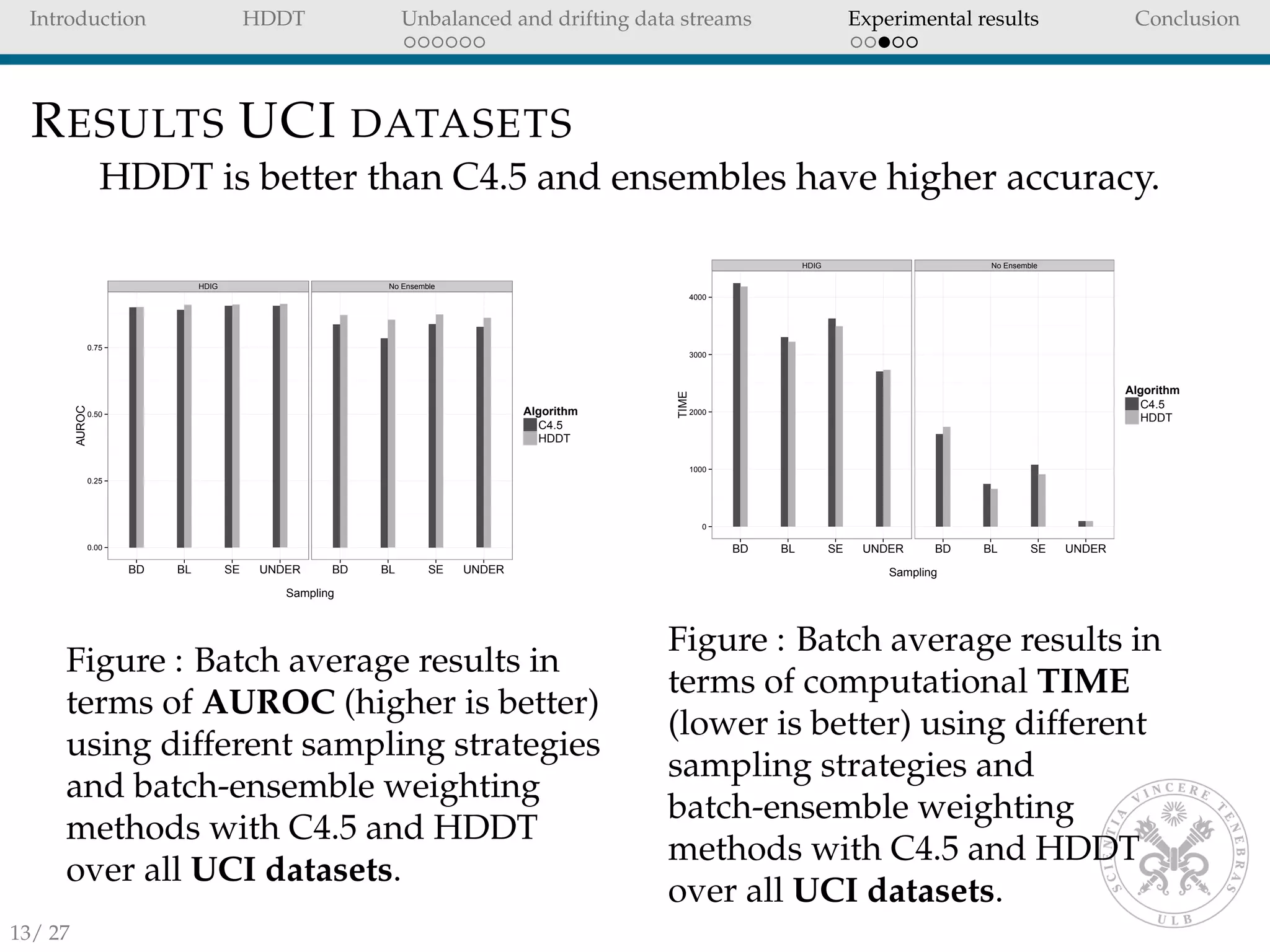
HDDT is better than C4.5 and ensembles have higher accuracy.
HDIG No Ensemble
0.00
0.25
0.50
0.75
BD BL SE UNDER BD BL SE UNDER
Sampling
AUROC
Algorithm
C4.5
HDDT
Figure : Batch average results in
terms of AUROC (higher is better)
using different sampling strategies
and batch-ensemble weighting
methods with C4.5 and HDDT
over all UCI datasets.
HDIG No Ensemble
0
1000
2000
3000
4000
BD BL SE UNDER BD BL SE UNDER
Sampling
TIME
Algorithm
C4.5
HDDT
Figure : Batch average results in
terms of computational TIME
(lower is better) using different
sampling strategies and
batch-ensemble weighting
methods with C4.5 and HDDT
over all UCI datasets.
13/ 27
Introduction HDDT Unbalanced and drifting data streams Experimental results Conclusion
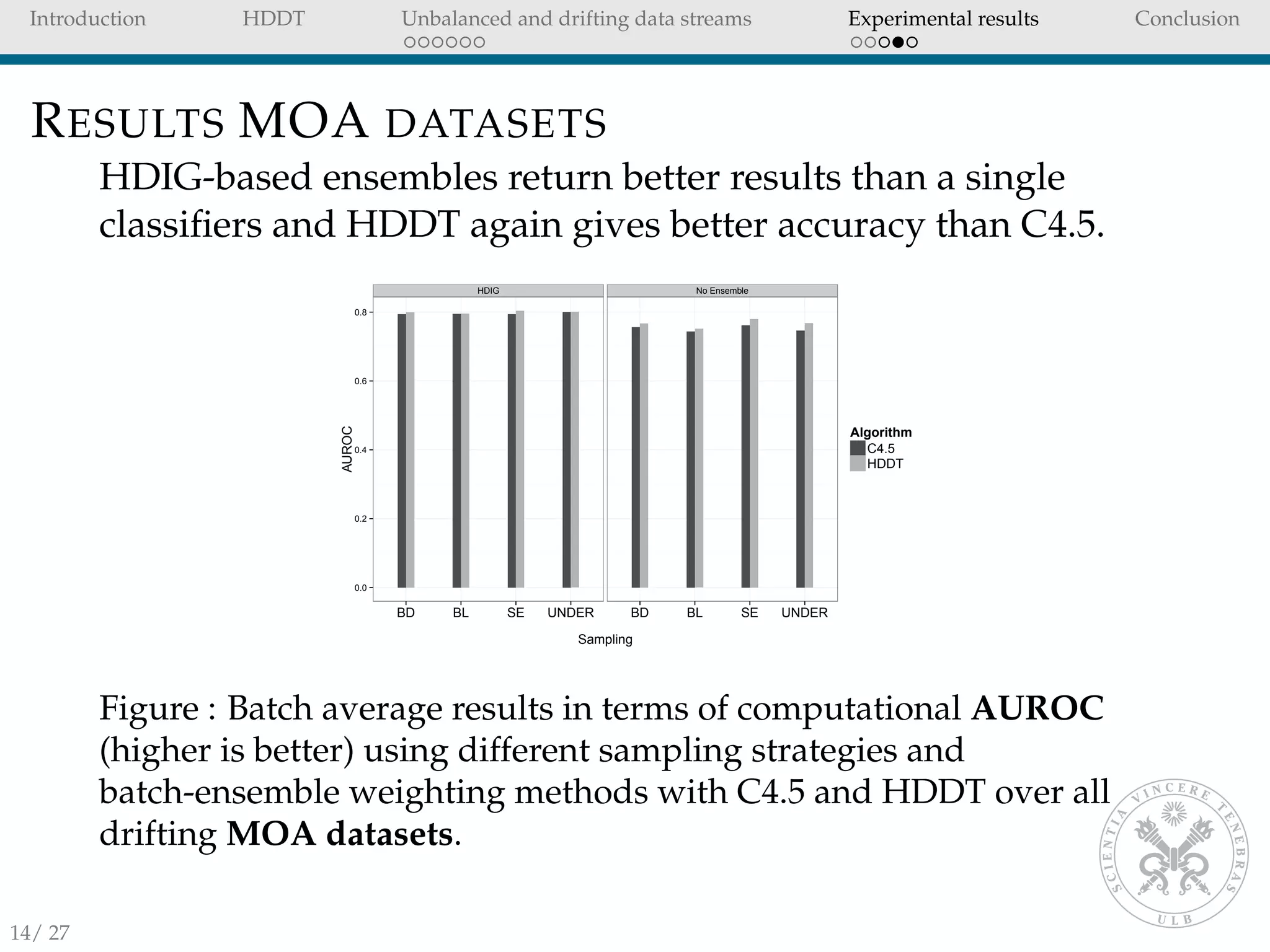
RESULTS MOA DATASETS
HDIG-based ensembles return better results than a single
classifiers and HDDT again gives better accuracy than C4.5.
HDIG No Ensemble
0.0
0.2
0.4
0.6
0.8
BD BL SE UNDER BD BL SE UNDER
Sampling
AUROC
Algorithm
C4.5
HDDT
Figure : Batch average results in terms of computational AUROC
(higher is better) using different sampling strategies and
batch-ensemble weighting methods with C4.5 and HDDT over all
drifting MOA datasets.
14/ 27
Introduction HDDT Unbalanced and drifting data streams Experimental results Conclusion
RESULTS CREDIT CARD DATASET
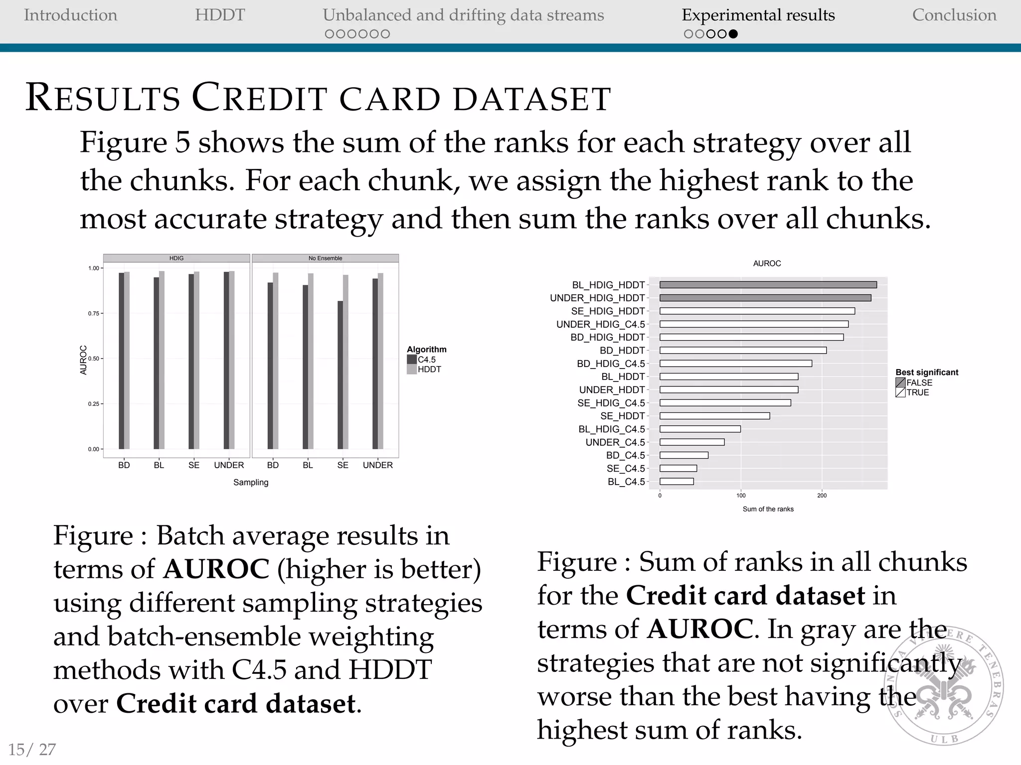
Figure 5 shows the sum of the ranks for each strategy over all
the chunks. For each chunk, we assign the highest rank to the
most accurate strategy and then sum the ranks over all chunks.
HDIG No Ensemble
0.00
0.25
0.50
0.75
1.00
BD BL SE UNDER BD BL SE UNDER
Sampling
AUROC
Algorithm
C4.5
HDDT
Figure : Batch average results in
terms of AUROC (higher is better)
using different sampling strategies
and batch-ensemble weighting
methods with C4.5 and HDDT
over Credit card dataset.
BL_C4.5
SE_C4.5
BD_C4.5
UNDER_C4.5
BL_HDIG_C4.5
SE_HDDT
SE_HDIG_C4.5
UNDER_HDDT
BL_HDDT
BD_HDIG_C4.5
BD_HDDT
BD_HDIG_HDDT
UNDER_HDIG_C4.5
SE_HDIG_HDDT
UNDER_HDIG_HDDT
BL_HDIG_HDDT
0 100 200
Sum of the ranks
Best significant
FALSE
TRUE
AUROC
Figure : Sum of ranks in all chunks
for the Credit card dataset in
terms of AUROC. In gray are the
strategies that are not significantly
worse than the best having the
highest sum of ranks.
15/ 27
Introduction HDDT Unbalanced and drifting data streams Experimental results Conclusion
CONCLUSION
In unbalanced data streams, state-of-the-art techniques use
instance propagation/sampling to deal with skewed
batches.
HDDT without sampling typically leads to better results
than C4.5 with sampling.
The removal of the propagation/sampling step in the
learning process has several benefits:
It allows a single-pass approach (avoids several passes
throughout the batches for instance propagation).
It reduces the computational cost (with massive amounts of
data it may no longer be possible to store/retrieve old
instances).
It avoids the problem of finding previous minority
instances from the same concept.
16/ 27
Introduction HDDT Unbalanced and drifting data streams Experimental results Conclusion
CONCLUSION II
HDIG ensemble weighting strategy:
has better performances than single classifiers.
takes into account drifts in the data stream.
With the credit card dataset HDDT performs very well
when combined with BL (no sampling) and UNDER
sampling.
These sampling strategies are the fastest, since no
observations are stored from previous chunks.
Future work will investigate propagation methods such as
REA [4], SERA [3] and HUWRS.IP [9] that are able to deal
with sub-concepts in the minority class.
THANK YOU FOR YOUR ATTENTION
17/ 27
Introduction HDDT Unbalanced and drifting data streams Experimental results Conclusion
BIBLIOGRAPHY I
D. N. A. Asuncion.
UCI machine learning repository, 2007.
A. Bifet, G. Holmes, R. Kirkby, and B. Pfahringer.
Moa: Massive online analysis.
The Journal of Machine Learning Research, 99:1601–1604, 2010.
S. Chen and H. He.
Sera: selectively recursive approach towards nonstationary imbalanced stream data mining.
In Neural Networks, 2009. IJCNN 2009. International Joint Conference on, pages 522–529. IEEE, 2009.
S. Chen and H. He.
Towards incremental learning of nonstationary imbalanced data stream: a multiple selectively recursive
approach.
Evolving Systems, 2(1):35–50, 2011.
D. A. Cieslak and N. V. Chawla.
Detecting fractures in classifier performance.
In Data Mining, 2007. ICDM 2007. Seventh IEEE International Conference on, pages 123–132. IEEE, 2007.
D. A. Cieslak and N. V. Chawla.
Learning decision trees for unbalanced data.
In Machine Learning and Knowledge Discovery in Databases, pages 241–256. Springer, 2008.
18/ 27
Introduction HDDT Unbalanced and drifting data streams Experimental results Conclusion
BIBLIOGRAPHY II
D. A. Cieslak, T. R. Hoens, N. V. Chawla, and W. P. Kegelmeyer.
Hellinger distance decision trees are robust and skew-insensitive.
Data Mining and Knowledge Discovery, 24(1):136–158, 2012.
J. Gao, B. Ding, W. Fan, J. Han, and P. S. Yu.
Classifying data streams with skewed class distributions and concept drifts.
Internet Computing, 12(6):37–49, 2008.
T. R. Hoens and N. V. Chawla.
Learning in non-stationary environments with class imbalance.
In Proceedings of the 18th ACM SIGKDD international conference on Knowledge discovery and data mining, pages
168–176. ACM, 2012.
T. R. Hoens, N. V. Chawla, and R. Polikar.
Heuristic updatable weighted random subspaces for non-stationary environments.
In Data Mining (ICDM), 2011 IEEE 11th International Conference on, pages 241–250. IEEE, 2011.
M. G. Kelly, D. J. Hand, and N. M. Adams.
The impact of changing populations on classifier performance.
In Proceedings of the fifth ACM SIGKDD international conference on Knowledge discovery and data mining, pages
367–371. ACM, 1999.
R. N. Lichtenwalter and N. V. Chawla.
Adaptive methods for classification in arbitrarily imbalanced and drifting data streams.
In New Frontiers in Applied Data Mining, pages 53–75. Springer, 2010.
19/ 27
Introduction HDDT Unbalanced and drifting data streams Experimental results Conclusion
BIBLIOGRAPHY III
J. R. Quinlan.
C4. 5: programs for machine learning, volume 1.
Morgan kaufmann, 1993.
C. R. Rao.
A review of canonical coordinates and an alternative to correspondence analysis using hellinger distance.
Questii´o: Quaderns d’Estad´ıstica, Sistemes, Informatica i Investigaci´o Operativa, 19(1):23–63, 1995.
20/ 27
Introduction HDDT Unbalanced and drifting data streams Experimental results Conclusion
HELLINGER DISTANCE
Quantify the similarity between two probability
distributions [14]
Recently proposed as a splitting criteria in decision trees
for unbalanced problems [6, 7].
In data streams, it has been used to detect classifier
performance degradation due to concept drift [5, 12].
21/ 27
Introduction HDDT Unbalanced and drifting data streams Experimental results Conclusion
HELLINGER DISTANCE II
Consider two probability measures P1, P2 of discrete
distributions in Φ. The Hellinger distance is defined as:
dH(P1, P2) =
φ∈Φ
P1(φ) − P2(φ)
2
(7)
Hellinger distance has several properties:
dH(P1, P2) = dH(P1, P2) (symmetric)
dH(P1, P2) >= 0 (non-negative)
dH(P1, P2) ∈ [0,
√
2]
dH is close to zero when the distributions are similar and close
to
√
2 for distinct distributions.
22/ 27
Introduction HDDT Unbalanced and drifting data streams Experimental results Conclusion
CONCEPT DRIFT II
Let us define Xt = {x0, x1, ..., xt} as the set of labeled
observations available at time t. For a new unlabelled instance
xt+1 we can train a classifier on Xt and predict P(ci|xt+1). Using
Bayes’ theorem we can write P(ci|xt+1) as:
P(ci|xt+1) =
P(ci)P(xt+1|ci)
P(xt+1)
(8)
Since P(xt+1) is the same for all classes ci we can remove
P(xt+1):
P(ci|xt+1) = P(ci)P(xt+1|ci) (9)
Kelly [11] argues that concept drift can occur from a change in
any of the terms in equation 9, namely:
P(ci), class priors.
P(xt+1|ci), distribution of the classes.
P(ci|xt+1), posterior distributions of class membership.
23/ 27
Introduction HDDT Unbalanced and drifting data streams Experimental results Conclusion
CONCEPT DRIFT III
The change in posterior distributions is the worst type of drift,
because it directly affects the performance of a classifier [9].
In general we don’t know where the changes in distributions
come from, but we can measure the distances between two
batches to estimate the similarities of the distributions.24/ 27

Using HDDT to avoid instances propagation in unbalanced and evolving data streams

  • 1.
    Introduction HDDT Unbalancedand drifting data streams Experimental results Conclusion Using HDDT to avoid instances propagation in unbalanced and evolving data streams IJCNN 2014 Andrea Dal Pozzolo, Reid Johnson, Olivier Caelen, Serge Waterschoot, Nitesh V Chawla and Gianluca Bontempi 07/07/2014 1/ 27
  • 2.
    Introduction HDDT Unbalancedand drifting data streams Experimental results Conclusion INTRODUCTION In many applications (e.g. Fraud detection), we have a stream of observations that we want to classify in real time. When one class is rare, the classification problem is said to be unbalanced. In this paper we focus unbalanced data stream with two classes, positive (minority) and negative (majority). In unbalanced data streams, state-of-the-art techniques use instance propagation and standard decision trees (e.g. C4.5 [13]). However, it is not always possible to either revisit or store old instances of a data stream. 2/ 27
  • 3.
    Introduction HDDT Unbalancedand drifting data streams Experimental results Conclusion INTRODUCTION II We use Hellinger Distance Decision Tree [7] (HDDT) to deal with skewed distributions in data streams. We consider data streams where the instances are received over time in streams of batches. HDDT allows us to remove instance propagations between batches, benefits: improved predictive accuracy speed single-pass through the data. An ensemble of HDDTs is used to combat concept drift and increase the accuracy of single classifiers. We test our framework on several streaming datasets with unbalanced classes and concept drift. 3/ 27
  • 4.
    Introduction HDDT Unbalancedand drifting data streams Experimental results Conclusion HELLINGER DISTANCE DECISION TREES HDDT [6] use Hellinger Distance as splitting criteria in decision trees for unbalanced problems. All numerical features are partitioned into p bins (only categorical variables). The Hellinger Distance between the positive and negative class is computed for each feature and then the feature with the maximum distance is used to split the tree. dH(f+, f−) = p j=1 |f+j| |f+| − |f−j| |f−| 2 (1) where f+ denote the positive instances and f− the negatives of feature f. Note that the class priors do not appear explicitly in equation 1. 4/ 27
  • 5.
    Introduction HDDT Unbalancedand drifting data streams Experimental results Conclusion CONCEPT DRIFT The concept to learn can change due to non-stationary distributions. In the presence of concept drift, we cannot longer assume that the training and testing batches come from the same distribution. Concept drift [11] can occur due to a change in: P(c), class priors. P(x|c), distribution of the classes. P(c|x), posterior distributions of class membership. 5/ 27
  • 6.
    Introduction HDDT Unbalancedand drifting data streams Experimental results Conclusion CONCEPT DRIFT II In general we don’t know where the changes in distributions come from, but we can measure the distances between two batches to estimate the similarities of the distributions. If the batch used for training a model is not similar to the testing batch, we can assume that the model is obsolete. In our work we use batch distances to assign low weights to obsolete models. 6/ 27
  • 7.
    Introduction HDDT Unbalancedand drifting data streams Experimental results Conclusion HELLINGER DISTANCE BETWEEN BATCHES Let Bt be the batch at time t used for training and Bt+1 the subsequent testing batch. We compute the distance between Bt and Bt+1 for a given feature f using Hellinger distance as proposed by Lichtenwalter and Chawla [12]: HD(Bt , Bt+1 , f) = v∈f   |Bt f=v| |Bt| − |Bt+1 f=v| |Bt+1|   2 (2) where |Bt f=v| is the number of instances of feature f taking value v in the batch at time t, while |Bt| is the total number of instances in the same batch. 7/ 27
  • 8.
    Introduction HDDT Unbalancedand drifting data streams Experimental results Conclusion INFORMATION GAIN Equation 2 does not account for differences in feature relevance. Lichtenwalter and Chawla [12] suggest to use the information gain to weight the distances. For a given feature f of a batch B, the Information Gain (IG) is defined as the decrease in entropy E of a class c: IG(B, f) = E(Bc) − E(Bc|Bf ) (3) where Bc defines the class of the observations in batch B and Bf the observations of feature f. 8/ 27
  • 9.
    Introduction HDDT Unbalancedand drifting data streams Experimental results Conclusion HELLINGER DISTANCE AND INFORMATION GAIN We can make the assumption that feature relevance remains stable over time and define a new distance function that combines IG and HD as: HDIG(Bt , Bt+1 , f) = HD(Bt , Bt+1 , f) ∗ (1 + IG(Bt , f)) (4) HDIG(Bt, Bt+1, f) provides a relevance-weighted distance for each single feature. The final distance between two batches is then computed taking the average over all the features. DHDIG(Bt , Bt+1 ) = f∈Bt HDIG(Bt, Bt+1, f) |f ∈ Bt| (5) 9/ 27
  • 10.
    Introduction HDDT Unbalancedand drifting data streams Experimental results Conclusion MODELS WEIGHTS In evolving data streams it is important to retain models learnt in the past and learn new models as soon as new data comes available. We learn a new model as soon as a new batch is available and store all the models. The learnt models are then combined into an ensemble where the weights are inversely proportional to the batches’ distances. The lower the distance between two batches the more similar is the concept between them. Lichtenwalter and Chawla [12] suggest to use the following transformation: weightst = 1 DHDIG(Bt, Bt+1)b (6) where b represents the ensemble size. 10/ 27
  • 11.
    Introduction HDDT Unbalancedand drifting data streams Experimental results Conclusion EXPERIMENTAL SETUP We compare HDDT with C4.5 [13] decision tree which is the standard for unbalanced data streams [10, 9, 12, 8]. We considered instance propagation methods that assume no sub-concepts within the minority class: SE (Gao’s [8] propagation of rare class instances and undersampling at 40%) BD (Lichtenwalter’s Boundary Definition [12]: propagating rare-class instances and instances in the negative class that the current model misclassifies.) UNDER (Undersampling: no propagation between batches, undersampling at 40%) BL (Baseline: no propagation, no sampling) For each of the previous sampling strategies we tested: HDIG: DHDIG weighted ensemble. No ensemble: single classifier. 11/ 27
  • 12.
    Introduction HDDT Unbalancedand drifting data streams Experimental results Conclusion DATASETS We used different types of datasets. UCI datasets [1] to first study the unbalanced problem without worrying about concept drift. Artificial datasets from MOA [2] framework with drifting features to test the behavior of the algorithms under concept drift. A credit card dataset (online payment transactions between the 5th of September and the 25th of September 2013). Name Source Instances Features Imbalance Ratio Adult UCI 48,842 14 3.2:1 can UCI 443,872 9 52.1:1 compustat UCI 13,657 20 27.5:1 covtype UCI 38,500 10 13.0:1 football UCI 4,288 13 1.7:1 ozone-8h UCI 2,534 72 14.8:1 wrds UCI 99,200 41 1.0:1 text UCI 11,162 11465 14.7:1 DriftedLED MOA 1,000,000 25 9.0:1 DriftedRBF MOA 1,000,000 11 1.02:1 DriftedWave MOA 1,000,000 41 2.02:1 Creditcard FRAUD 3,143,423 36 658.8:1 12/ 27
  • 13.
    Introduction HDDT Unbalancedand drifting data streams Experimental results Conclusion RESULTS UCI DATASETS HDDT is better than C4.5 and ensembles have higher accuracy. HDIG No Ensemble 0.00 0.25 0.50 0.75 BD BL SE UNDER BD BL SE UNDER Sampling AUROC Algorithm C4.5 HDDT Figure : Batch average results in terms of AUROC (higher is better) using different sampling strategies and batch-ensemble weighting methods with C4.5 and HDDT over all UCI datasets. HDIG No Ensemble 0 1000 2000 3000 4000 BD BL SE UNDER BD BL SE UNDER Sampling TIME Algorithm C4.5 HDDT Figure : Batch average results in terms of computational TIME (lower is better) using different sampling strategies and batch-ensemble weighting methods with C4.5 and HDDT over all UCI datasets. 13/ 27
  • 14.
    Introduction HDDT Unbalancedand drifting data streams Experimental results Conclusion RESULTS MOA DATASETS HDIG-based ensembles return better results than a single classifiers and HDDT again gives better accuracy than C4.5. HDIG No Ensemble 0.0 0.2 0.4 0.6 0.8 BD BL SE UNDER BD BL SE UNDER Sampling AUROC Algorithm C4.5 HDDT Figure : Batch average results in terms of computational AUROC (higher is better) using different sampling strategies and batch-ensemble weighting methods with C4.5 and HDDT over all drifting MOA datasets. 14/ 27
  • 15.
    Introduction HDDT Unbalancedand drifting data streams Experimental results Conclusion RESULTS CREDIT CARD DATASET Figure 5 shows the sum of the ranks for each strategy over all the chunks. For each chunk, we assign the highest rank to the most accurate strategy and then sum the ranks over all chunks. HDIG No Ensemble 0.00 0.25 0.50 0.75 1.00 BD BL SE UNDER BD BL SE UNDER Sampling AUROC Algorithm C4.5 HDDT Figure : Batch average results in terms of AUROC (higher is better) using different sampling strategies and batch-ensemble weighting methods with C4.5 and HDDT over Credit card dataset. BL_C4.5 SE_C4.5 BD_C4.5 UNDER_C4.5 BL_HDIG_C4.5 SE_HDDT SE_HDIG_C4.5 UNDER_HDDT BL_HDDT BD_HDIG_C4.5 BD_HDDT BD_HDIG_HDDT UNDER_HDIG_C4.5 SE_HDIG_HDDT UNDER_HDIG_HDDT BL_HDIG_HDDT 0 100 200 Sum of the ranks Best significant FALSE TRUE AUROC Figure : Sum of ranks in all chunks for the Credit card dataset in terms of AUROC. In gray are the strategies that are not significantly worse than the best having the highest sum of ranks. 15/ 27
  • 16.
    Introduction HDDT Unbalancedand drifting data streams Experimental results Conclusion CONCLUSION In unbalanced data streams, state-of-the-art techniques use instance propagation/sampling to deal with skewed batches. HDDT without sampling typically leads to better results than C4.5 with sampling. The removal of the propagation/sampling step in the learning process has several benefits: It allows a single-pass approach (avoids several passes throughout the batches for instance propagation). It reduces the computational cost (with massive amounts of data it may no longer be possible to store/retrieve old instances). It avoids the problem of finding previous minority instances from the same concept. 16/ 27
  • 17.
    Introduction HDDT Unbalancedand drifting data streams Experimental results Conclusion CONCLUSION II HDIG ensemble weighting strategy: has better performances than single classifiers. takes into account drifts in the data stream. With the credit card dataset HDDT performs very well when combined with BL (no sampling) and UNDER sampling. These sampling strategies are the fastest, since no observations are stored from previous chunks. Future work will investigate propagation methods such as REA [4], SERA [3] and HUWRS.IP [9] that are able to deal with sub-concepts in the minority class. THANK YOU FOR YOUR ATTENTION 17/ 27
  • 18.
    Introduction HDDT Unbalancedand drifting data streams Experimental results Conclusion BIBLIOGRAPHY I D. N. A. Asuncion. UCI machine learning repository, 2007. A. Bifet, G. Holmes, R. Kirkby, and B. Pfahringer. Moa: Massive online analysis. The Journal of Machine Learning Research, 99:1601–1604, 2010. S. Chen and H. He. Sera: selectively recursive approach towards nonstationary imbalanced stream data mining. In Neural Networks, 2009. IJCNN 2009. International Joint Conference on, pages 522–529. IEEE, 2009. S. Chen and H. He. Towards incremental learning of nonstationary imbalanced data stream: a multiple selectively recursive approach. Evolving Systems, 2(1):35–50, 2011. D. A. Cieslak and N. V. Chawla. Detecting fractures in classifier performance. In Data Mining, 2007. ICDM 2007. Seventh IEEE International Conference on, pages 123–132. IEEE, 2007. D. A. Cieslak and N. V. Chawla. Learning decision trees for unbalanced data. In Machine Learning and Knowledge Discovery in Databases, pages 241–256. Springer, 2008. 18/ 27
  • 19.
    Introduction HDDT Unbalancedand drifting data streams Experimental results Conclusion BIBLIOGRAPHY II D. A. Cieslak, T. R. Hoens, N. V. Chawla, and W. P. Kegelmeyer. Hellinger distance decision trees are robust and skew-insensitive. Data Mining and Knowledge Discovery, 24(1):136–158, 2012. J. Gao, B. Ding, W. Fan, J. Han, and P. S. Yu. Classifying data streams with skewed class distributions and concept drifts. Internet Computing, 12(6):37–49, 2008. T. R. Hoens and N. V. Chawla. Learning in non-stationary environments with class imbalance. In Proceedings of the 18th ACM SIGKDD international conference on Knowledge discovery and data mining, pages 168–176. ACM, 2012. T. R. Hoens, N. V. Chawla, and R. Polikar. Heuristic updatable weighted random subspaces for non-stationary environments. In Data Mining (ICDM), 2011 IEEE 11th International Conference on, pages 241–250. IEEE, 2011. M. G. Kelly, D. J. Hand, and N. M. Adams. The impact of changing populations on classifier performance. In Proceedings of the fifth ACM SIGKDD international conference on Knowledge discovery and data mining, pages 367–371. ACM, 1999. R. N. Lichtenwalter and N. V. Chawla. Adaptive methods for classification in arbitrarily imbalanced and drifting data streams. In New Frontiers in Applied Data Mining, pages 53–75. Springer, 2010. 19/ 27
  • 20.
    Introduction HDDT Unbalancedand drifting data streams Experimental results Conclusion BIBLIOGRAPHY III J. R. Quinlan. C4. 5: programs for machine learning, volume 1. Morgan kaufmann, 1993. C. R. Rao. A review of canonical coordinates and an alternative to correspondence analysis using hellinger distance. Questii´o: Quaderns d’Estad´ıstica, Sistemes, Informatica i Investigaci´o Operativa, 19(1):23–63, 1995. 20/ 27
  • 21.
    Introduction HDDT Unbalancedand drifting data streams Experimental results Conclusion HELLINGER DISTANCE Quantify the similarity between two probability distributions [14] Recently proposed as a splitting criteria in decision trees for unbalanced problems [6, 7]. In data streams, it has been used to detect classifier performance degradation due to concept drift [5, 12]. 21/ 27
  • 22.
    Introduction HDDT Unbalancedand drifting data streams Experimental results Conclusion HELLINGER DISTANCE II Consider two probability measures P1, P2 of discrete distributions in Φ. The Hellinger distance is defined as: dH(P1, P2) = φ∈Φ P1(φ) − P2(φ) 2 (7) Hellinger distance has several properties: dH(P1, P2) = dH(P1, P2) (symmetric) dH(P1, P2) >= 0 (non-negative) dH(P1, P2) ∈ [0, √ 2] dH is close to zero when the distributions are similar and close to √ 2 for distinct distributions. 22/ 27
  • 23.
    Introduction HDDT Unbalancedand drifting data streams Experimental results Conclusion CONCEPT DRIFT II Let us define Xt = {x0, x1, ..., xt} as the set of labeled observations available at time t. For a new unlabelled instance xt+1 we can train a classifier on Xt and predict P(ci|xt+1). Using Bayes’ theorem we can write P(ci|xt+1) as: P(ci|xt+1) = P(ci)P(xt+1|ci) P(xt+1) (8) Since P(xt+1) is the same for all classes ci we can remove P(xt+1): P(ci|xt+1) = P(ci)P(xt+1|ci) (9) Kelly [11] argues that concept drift can occur from a change in any of the terms in equation 9, namely: P(ci), class priors. P(xt+1|ci), distribution of the classes. P(ci|xt+1), posterior distributions of class membership. 23/ 27
  • 24.
    Introduction HDDT Unbalancedand drifting data streams Experimental results Conclusion CONCEPT DRIFT III The change in posterior distributions is the worst type of drift, because it directly affects the performance of a classifier [9]. In general we don’t know where the changes in distributions come from, but we can measure the distances between two batches to estimate the similarities of the distributions.24/ 27