Download as PDF, PPTX
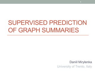


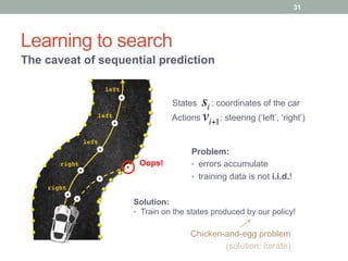
![Searn and DAGGER
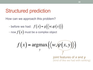
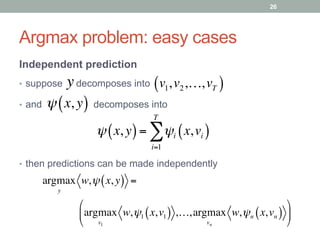
Searn = “search” + “learn”
• start from optimal policy;
move away
• generate new states with current
• generate actions based on regret
• train on new state-action pairs
• interpolate the current policy
πi+1 ← βπi + 1− β( ) #πi+1
policy learnt at ith iteration
regret
32
[1] Hal Daumé III, John Langford, Daniel Marcu. Search-based Structured Prediction. Machine Learning Journal, 2006.
[1]
!πi+1
πi](https://image.slidesharecdn.com/supervisedpredictionofgraphsummariesgoogle-141018062403-conversion-gate01/85/Supervised-Prediction-of-Graph-Summaries-32-320.jpg)
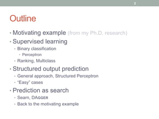
![Searn and DAGGER
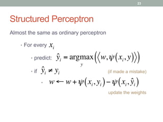
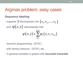
DAGGER = “dataset” + “aggregation”
• start from the ‘ground truth’ dataset,
enrich it with new state-action pairs
• train a policy on the current dataset
• use the policy to generate new states
• generate ‘expert’s actions’ for new states
• add new state-action pairs to the dataset
expert’s
actions
As in Searn, we’ll eventually be training
on our own-produced states
33
[2] Stephane Ross, Geoffrey Gordon, Drew Bagnell. A reduction of imitation learning and
structured prediction to no-regret online learning. Journal of Machine Learning Research, 2011.
[2]](https://image.slidesharecdn.com/supervisedpredictionofgraphsummariesgoogle-141018062403-conversion-gate01/85/Supervised-Prediction-of-Graph-Summaries-33-320.jpg)
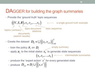
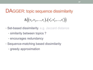
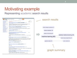
![DAGGER: topic graph features
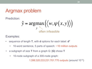
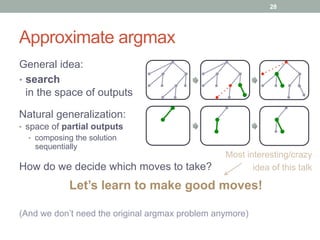
• Coverage and diversity
• [transitive] document coverage
• [transitive] topic frequency, average and min
• topic overlap, average and max
• parent-child overlap, average and max
• …
38
ψ V,S, R( ), v1,v2,…,vt( )( )](https://image.slidesharecdn.com/supervisedpredictionofgraphsummariesgoogle-141018062403-conversion-gate01/85/Supervised-Prediction-of-Graph-Summaries-38-320.jpg)


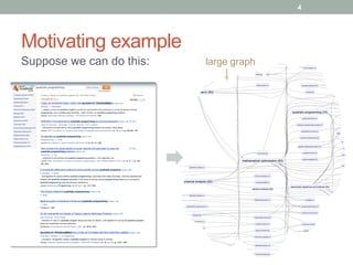
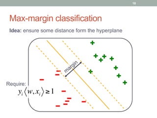
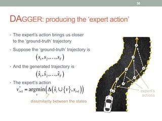
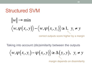
![Support Vector Machine
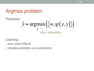
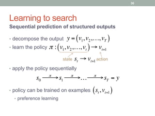
Idea: large margin between positive and negative examples
Loss function:
L y, f x( )( )=[1− y⋅ f x( )]+
Hinge loss
(solved by constrained convex optimization)
yi w, xi ≥ C
C → max
#
$
%
&%
⇔
yi w, xi ≥1
w → min
#
$
%
&%
42](https://image.slidesharecdn.com/supervisedpredictionofgraphsummariesgoogle-141018062403-conversion-gate01/85/Supervised-Prediction-of-Graph-Summaries-42-320.jpg)

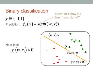
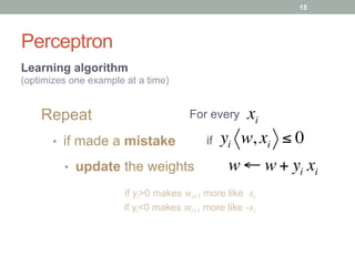
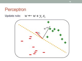
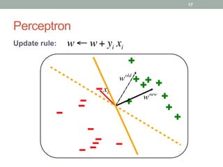
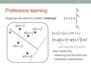
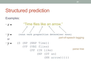
The document discusses the supervised prediction of graph summaries, focusing on various machine learning techniques such as binary classification, ranking, and structured output prediction. It highlights methods like the perceptron algorithm, structured perceptron, and learning to search through approaches like SEARN and DAgger for efficient predictions and decision-making in complex structured outputs. The conclusion outlines how these techniques can apply to fine-tuning predictions based on ground truth representations in graph summarization tasks.