Downloaded 1,798 times


![5
analytical disciplines, such as descriptive modeling and decision
modeling or optimization. These disciplines also involve rigorous data
analysis, and are widely used in business for segmentation and decision
making, but have different purposes and the statistical techniques
underlying them vary.
Predictive models
Predictive models are models of the relation between the specific
performance of a unit in a sample and one or more known attributes or
features of the unit. The objective of the model is to assess the likelihood
that a similar unit in a different sample will exhibit the specific
performance. This category encompasses models that are in many areas,
such as marketing, where they seek out subtle data patterns to answer
questions about customer performance, such as fraud detection models.
Predictive models often perform calculations during live transactions,
for example, to evaluate the risk or opportunity of a given customer or
transaction, in order to guide a decision. With advancements in
computing speed, individual agent modeling systems have become
capable of simulating human behavior or reactions to given stimuli or
scenarios.
The available sample units with known attributes and known
performances is referred to as the “training sample.” The units in other
sample, with known attributes but un-known performances, are
referred to as “out of [training] sample” units. The out of sample bear
no chronological relation to the training sample units. For example, the
training sample may consists of literary attributes of writings by
Victorian authors, with known attribution, and the out-of sample unit
may be newly found writing with unknown authorship; a predictive
model may aid the attribution of the unknown author. Another example
is given by analysis of blood splatter in simulated crime scenes in which
the out-of sample unit is the actual blood splatter pattern from a crime
scene. The out of sample unit may be from the same time as the training
units, from a previous time, or from a future time.](https://image.slidesharecdn.com/048d9789-800e-4318-80f7-c96b1a8df646-150122193330-conversion-gate01/85/Predictive-Analytics-using-R-36-320.jpg)


![39
http://cran.r-project.org/mirrors.html. You should pick your nearest
location.
Using External Data. R offers plenty of options for loading external
data, including Excel, Minitab and SPSS files.
R Session. After R is started, there is a console awaiting for input. At
the prompt (>), you can enter numbers and perform calculations.
> 1 + 2
[1] 3
Variable Assignment. We assign values to variables with the
assignment operator “=“. Just typing the variable by itself at the
prompt will print out the value. We should note that another form of
assignment operator “<-” is also in use.
> x = 1
> x
[1] 1
Functions. R functions are invoked by its name, then followed by the
parenthesis, and zero or more arguments. The following apply the
function c to combine three numeric values into a vector.
> c(1, 2, 3)
[1] 1 2 3
Comments. All text after the pound sign “#” within the same line is
considered a comment.
> 1 + 1 # this is a comment
[1] 2
Extension Package. Sometimes we need additional functionality
beyond those offered by the core R library. In order to install an
extension package, you should invoke the install.packages function at
the prompt and follow the instruction.](https://image.slidesharecdn.com/048d9789-800e-4318-80f7-c96b1a8df646-150122193330-conversion-gate01/85/Predictive-Analytics-using-R-70-320.jpg)
![40
> install.packages()
Getting Help. R provides extensive documentation. For example,
entering ?c or help(c) at the prompt gives documentation of the
function c in R.
> help(c)
If you are not sure about the name of the function you are looking for,
you can perform a fuzzy search with the apropos function.
> apropos(“nova”)
[1] “anova” “anova.glm”
....
Finally, there is an R specific Internet search engine at
http://www.rseek.org for more assistance.](https://image.slidesharecdn.com/048d9789-800e-4318-80f7-c96b1a8df646-150122193330-conversion-gate01/85/Predictive-Analytics-using-R-71-320.jpg)


![56
𝐸(𝜃𝑖|𝑦𝑖) =
(𝑦𝑖 + 1)𝑝 𝐺(𝑦𝑖 + 1)
𝑝 𝐺(𝑦𝑖)
,
where 𝑝 𝐺 is the marginal distribution obtained by integrating out 𝜃 over
𝐺 (Wald, 1971).
To take advantage of this, Robbins (Robbins, 1956) suggested estimating
the marginals with their empirical frequencies, yielding the fully non-
parametric estimate as:
𝐸(𝜃𝑖|𝑦𝑖) = (𝑦𝑖 + 1)
#{𝑌𝑗 = 𝑦𝑖 + 1}
#{𝑌𝑗 = 𝑦𝑖}
,
where # denotes “number of” (Good, 1953).
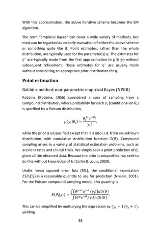
Example - Accident rates
Suppose each customer of an insurance company has an “accident rate”
𝛩 and is insured against accidents; the probability distribution of 𝛩 is the
underlying distribution, and is unknown. The number of accidents
suffered by each customer in a specified time period has a Poisson
distribution with expected value equal to the particular customer’s
accident rate. The actual number of accidents experienced by a
customer is the observable quantity. A crude way to estimate the
underlying probability distribution of the accident rate 𝛩 is to estimate
the proportion of members of the whole population suffering
0, 1, 2, 3, … accidents during the specified time period as the
corresponding proportion in the observed random sample. Having done
so, we then desire to predict the accident rate of each customer in the
sample. As above, one may use the conditional expected value of the
accident rate 𝛩 given the observed number of accidents during the
baseline period. Thus, if a customer suffers six accidents during the
baseline period, that customer’s estimated accident rate is
7 × [𝑡ℎ𝑒 𝑝𝑟𝑜𝑝𝑜𝑟𝑡𝑖𝑜𝑛 𝑜𝑓 𝑡ℎ𝑒 𝑠𝑎𝑚𝑝𝑙𝑒 𝑤ℎ𝑜 𝑠𝑢𝑓𝑓𝑒𝑟𝑒𝑑 7 𝑎𝑐𝑐𝑖𝑑𝑒𝑛𝑡𝑠] /
[𝑡ℎ𝑒 𝑝𝑟𝑜𝑝𝑜𝑟𝑡𝑖𝑜𝑛 𝑜𝑓 𝑡ℎ𝑒 𝑠𝑎𝑚𝑝𝑙𝑒 𝑤ℎ𝑜 𝑠𝑢𝑓𝑓𝑒𝑟𝑒𝑑 6 𝑎𝑐𝑐𝑖𝑑𝑒𝑛𝑡𝑠].
Note that if the proportion of people suffering 𝑘 accidents is a](https://image.slidesharecdn.com/048d9789-800e-4318-80f7-c96b1a8df646-150122193330-conversion-gate01/85/Predictive-Analytics-using-R-87-320.jpg)


![59
explicit results are available for the posterior probability distributions of
the model’s parameters.
Consider a standard linear regression problem, in which for 𝑖 = 1, . . . , 𝑛.
We specify the conditional distribution of 𝒚𝑖 given a 𝑘 × 1 predictor
vector 𝒙𝒊:
𝒚𝑖 = 𝑿𝑖
𝑇
𝜷 + 𝜀𝑖,
where 𝜷 is a 𝑘 × 1 vector, and the 𝜀𝑖 are independent and identical
normally distributed random variables:
𝜀𝑖~𝑁(𝜇, 𝜎2).
This corresponds to the following likelihood function:
𝜌(𝒚|𝑿, 𝜷, 𝜎2) ∝ (𝜎2)−𝑛 2⁄
exp (−
1
2𝜎2
(𝒚 − 𝑿𝜷) 𝑇(𝒚 − 𝑿𝜷)) .
The ordinary least squares solution is to estimate the coefficient vector
using the Moore-Penrose pseudoinverse (Penrose, 1955) (Ben-Israel &
Greville, 2003):
𝜷̂ = (𝑿 𝑇
𝑿)−1
𝑿 𝑇
𝒚,
Where 𝑿 is the 𝑛 × 𝑘 design matrix, each row of which is a predictor
vector 𝑿𝑖
𝑇
; and 𝒚 is the column 𝑛-vector [ 𝑦1 ⋯ 𝑦𝑛] 𝑇
.
This is a “frequentist” approach (Neyman, 1937), and it assumes that
there are enough measurements to say something meaningful about 𝜷.
In the Bayesian approach, the data are supplemented with additional
information in the form of a prior probability distribution. The prior
belief about the parameters is combined with the data’s likelihood
function according to Bayes theorem to yield the posterior belief about
the parameters 𝜷 and 𝜎. The prior can take different functional forms
depending on the domain and the information that is available a priori.](https://image.slidesharecdn.com/048d9789-800e-4318-80f7-c96b1a8df646-150122193330-conversion-gate01/85/Predictive-Analytics-using-R-90-320.jpg)
![60
Software
Several software packages are available that perform Empirical Bayes,
including the Open Source software R with the limma package. Tos start
the package in R, one simply enters the following in the R console at the
prompt
>
source(“http://bioconductor.org/biocLite.R”)biocLite(“limma
”).
Commercial software includes MATLAB, SAS and SPSS.
Example Using R
Model Selection in Bayesian Linear Regression
Consider data generated by 𝑦𝑖 = 𝑏1 𝑥𝑖 + 𝑏3 𝑥𝑖
3
+ 𝜀𝑖, and suppose we
wish to fit a polynomial of degree 3 to the data. There are then 4
regression coefficients, namely, the intercept and the three coefficients
of the power of x. This yields 24
= 16 models possible models for the
data. Let 𝑏1 = 8 and 𝑏3 = −0.5 so that the data looks like this in R:
> rm(list=ls())
> x=runif(200,-10,10)
> a=c(18,0,-0.5,0)
> Y=a[1]*x^1+a[2]*x^2+a[3]*x^3+a[4]
> Y=Y+rnorm(length(Y),0,5)
> plot(x,Y)](https://image.slidesharecdn.com/048d9789-800e-4318-80f7-c96b1a8df646-150122193330-conversion-gate01/85/Predictive-Analytics-using-R-91-320.jpg)
![61
The code to generate the data and calculate the log marginal likelihood
for the different models appears below.
> p=4
> X=cbind(x,x^2,x^3,1)
> tf <- c(TRUE, FALSE)
> models <- expand.grid(replicate(p,tf,simplify=FALSE))
> names(models) <- NULL
> models=as.matrix(models)
> models=models[-dim(models)[1],]
> a_0=100
> b_0=0.5
> mu_0=rep(0,p)
> lambda_0=diag(p)
> lml <- function(model){
+ n=length(Y)
+ Y=as.matrix(Y)
+ X=as.matrix(X[,model])
+ mu_0=as.matrix(mu_0[model])](https://image.slidesharecdn.com/048d9789-800e-4318-80f7-c96b1a8df646-150122193330-conversion-gate01/85/Predictive-Analytics-using-R-92-320.jpg)
![62
+ lambda_0=as.matrix(lambda_0[model,model])
+ XtX=t(X)%*%X
+ lambda_n=lambda_0 + XtX
+ BMLE=solve(XtX)%*%t(X)%*%Y
+ mu_n=solve(lambda_n)%*%(t(X)%*%Y+lambda_0%*%mu_0)
+ a_n = a_0 + 0.5*n
+ b_n=b_0 + 0.5*(t(Y)%*%Y + t(mu_0)%*%lambda_0%*%mu_0 –
+ t(mu_n)%*%lambda_n%*%mu_n)
+ log_mar_lik <- -0.5*n*log(2*pi) +
+ 0.5*log(det(lambda_0)) - 0.5*log(det(lambda_n)) +
+ lgamma(a_n) - lgamma(a_0) + a_0*log(b_0) –
+ a_n*log(b_n)
+ return(mle)
+ }
> lml.all=apply(models,1,lml)
> results=cbind(lml.all, models)
> order=sort(results[,1],index=TRUE,decreasing=TRUE)
> results[order$ix,]
Model Evaluation
The models are listed in order of descending log marginal likelihood
below:
lml x x^2 x^3 c
[1,] -1339.085 1 0 1 0
[2,] -1341.611 1 0 1 1
[3,] -1345.397 1 1 1 0
[4,] -1347.116 1 1 1 1
[5,] -2188.934 0 0 1 0
[6,] -2190.195 0 0 1 1
[7,] -2194.238 0 1 1 0
[8,] -2196.109 0 1 1 1
[9,] -2393.395 1 0 0 0
[10,] -2395.309 1 0 0 1
[11,] -2399.188 1 1 0 0
[12,] -2401.248 1 1 0 1
[13,] -2477.084 0 0 0 1
[14,] -2480.784 0 1 0 0
[15,] -2483.047 0 1 0 1](https://image.slidesharecdn.com/048d9789-800e-4318-80f7-c96b1a8df646-150122193330-conversion-gate01/85/Predictive-Analytics-using-R-93-320.jpg)
![63
> BMLE
[,1]
x 18.241814068
0.008942083
-0.502597759
-0.398375650
The model with the highest log marginal likelihood is the model which
includes 𝑥 and 𝑥3
only, for which the MLE of the regression coefficients
are 18.241814068 and -0.502597759 for 𝑥 and 𝑥3
respectively.
Compare this to how the data was generated.](https://image.slidesharecdn.com/048d9789-800e-4318-80f7-c96b1a8df646-150122193330-conversion-gate01/85/Predictive-Analytics-using-R-94-320.jpg)


![71
Bernoulli Naïve Bayes
In the multivariate Bernoulli event model, features are independent
Booleans (binary variables) describing inputs. This model is also popular
for document classification tasks, where binary term occurrence
features are used rather than term frequencies. If 𝐹𝑖 is a Boolean
expressing the occurrence or absence of the 𝑖-th term from the
vocabulary, then the likelihood of a document given a class 𝐶 is given by
𝑝(𝐹1, … , 𝐹𝑛|𝐶) = ∏[𝐹𝑖 𝑝(𝑤𝑖|𝐶) + (1 − 𝐹𝑖)(1 − 𝑝(𝑤𝑖|𝐶))]
𝑛
𝑖=1
where 𝑝(𝑤𝑖|𝐶) is the probability of class 𝐶 generating the term 𝑤𝑖. This
event model is especially popular for classifying short texts. It has the
benefit of explicitly modeling the absence of terms. Note that a Naïve
Bayes classifier with a Bernoulli event model is not the same as a
multinomial NB classifier with frequency counts truncated to one.
Discussion
Despite the fact that the far-reaching independence assumptions are
often inaccurate, the Naïve Bayes classifier has several properties that
make it surprisingly useful in practice. In particular, the decoupling of the
class conditional feature distributions means that each distribution can
be independently estimated as a one-dimensional distribution. This
helps alleviate problems stemming from the curse of dimensionality,
such as the need for data sets that scale exponentially with the number
of features. While Naïve Bayes often fails to produce a good estimate for
the correct class probabilities, this may not be a requirement for many
applications. For example, the Naïve Bayes classifier will make the
correct MAP decision rule classification so long as the correct class is
more probable than any other class. This is true regardless of whether
the probability estimate is slightly, or even grossly inaccurate. In this
manner, the overall classifier can be robust enough to ignore serious
deficiencies in its underlying naive probability model. Other reasons for
the observed success of the Naïve Bayes classifier are discussed in the](https://image.slidesharecdn.com/048d9789-800e-4318-80f7-c96b1a8df646-150122193330-conversion-gate01/85/Predictive-Analytics-using-R-102-320.jpg)


![78
programming rules-based environment.
Netica – by NORSYS, is Bayesian network development software
provides Bayesian network tools.
PrecisionTree – by Paslisade (makers of @Risk), is an add-in for
Microsoft Excel for building decision trees and influence diagrams
directly in the spreadsheet
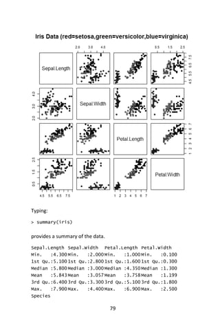
Example Using R
The Iris dataset is pre-installed in R, since it is in the standard datasets
package. To access its documentation, click on ‘Packages’ at the top-
level of the R documentation, then on ‘datasets’ and then on ‘iris’. As
explained, there are 150 data points and 5 variables. Each data point
concerns a particular iris flower and gives 4 measurements of the flower:
Sepal.Length, Sepal.Width, Petal.Length and Petal.Width together
with the flower’s Species. The goal is to build a classifier that predicts
species from the 4 measurements, so species is the class variable.
To get the iris dataset into your R session, do:
> data(iris)
at the R prompt. As always, it makes sense to look at the data. The
following R command (from the Wikibook) does a nice job of this.
> pairs(iris[1:4],main=“Iris Data
+ (red=setosa,green=versicolor,blue=virginica)”, pch=21,
+ bg=c(“red”,”green3”,”blue”)[unclass(iris$Species)])
The ‘pairs’ command creates a scatterplot. Each dot is a data point and
its position is determined by the values that data point has for a pair of
variables. The class determines the color of the data point. From the plot
note that Setosa irises have smaller petals than the other two species.](https://image.slidesharecdn.com/048d9789-800e-4318-80f7-c96b1a8df646-150122193330-conversion-gate01/85/Predictive-Analytics-using-R-109-320.jpg)

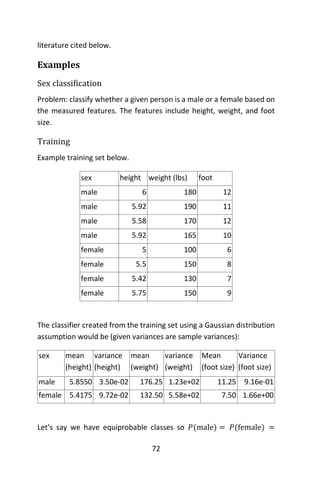
![81
To (1) load e1071 into your workspace (2) build a Naïve Bayes classifier
and (3) make some predictions on the training data, do:
> library(e1071)
> classifier<-naiveBayes(iris[,1:4], iris[,5])
> table(predict(classifier, iris[,-5]), iris[,5],
+ dnn=list(‘predicted’,’actual’))
As you should see the classifier does a pretty good job of classifying. Why
is this not surprising?
predicted setosa versicolor virginica
setosa 50 0 0
versicolor 0 47 3
virginica 0 3 47
To see what’s going on ‘behind-the-scenes’, first do:
> classifier$apriori
This gives the class distribution in the data: the prior distribution of the
classes. (‘A priori’ is Latin for ‘from before’.)
iris[, 5]
setosa versicolor virginica
50 50 50
Since the predictor variables here are all continuous, the Naïve Bayes
classifier generates three Gaussian (Normal) distributions for each
predictor variable: one for each value of the class variable Species. If you
type:
> classifier$tables$Petal.Length
You will see the mean (first column) and standard deviation (second
column) for the 3 class-dependent Gaussian distributions:
Petal.Length
iris[, 5] [,1] [,2]
setosa 1.462 0.1736640](https://image.slidesharecdn.com/048d9789-800e-4318-80f7-c96b1a8df646-150122193330-conversion-gate01/85/Predictive-Analytics-using-R-112-320.jpg)


![96
Examples Using R
Classification Tree example
Let’s use the data frame kyphosis to predict a type of deformation
(kyphosis) after surgery, from age in months (Age), number of vertebrae
involved (Number), and the highest vertebrae operated on (Start).
In R, call the rpart library. Recursive partitioning for classification,
regression and survival trees. An implementation of most of the
functionality of the 1984 book by Breiman, Friedman, Olshen and Stone
(Breiman, Friedman, Olshen, & Stone, 1984).
# Classification Tree with rpart
> library(rpart)
We will not grow the tree with the fit() and rpart functions.
# grow tree
> fit <- rpart(Kyphosis ~ Age + Number + Start,
+ method=“class”, data=kyphosis)
where kyphosis is the response, with variables Age, Number, and Start.
Class in the method and kyphosis is the data set. Next, we display the
results.
> printcp(fit) # display the results
Classification tree:
rpart(formula = Kyphosis~Age + Number + Start, data =
kyphosis,
method = “class”)
Variables actually used in tree construction:
[1] Age Start
Root node error: 17/81 = 0.20988
n= 81
CP nsplit rel error xerror xstd](https://image.slidesharecdn.com/048d9789-800e-4318-80f7-c96b1a8df646-150122193330-conversion-gate01/85/Predictive-Analytics-using-R-127-320.jpg)


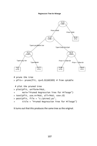
![102
We now “prune” the tree and display its plot.
# prune the tree
> Pfit <- prune(fit,cp= fit$cptable [which.min(
+ fit$cptable[,”xerror”]),”CP”])
# plot the pruned tree
> plot(pfit, uniform=TRUE,
+ main=“Pruned Classification Tree for Kyphosis”)
> text(pfit, use.n=TRUE, all=TRUE, cex=.8)
> post(pfit, file = “c:/ptree.ps”,
+ title = “Pruned Classification Tree for Kyphosis”)](https://image.slidesharecdn.com/048d9789-800e-4318-80f7-c96b1a8df646-150122193330-conversion-gate01/85/Predictive-Analytics-using-R-133-320.jpg)


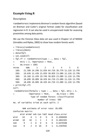
![120
Tabl 0 1 0 0 8 0 0.1111111
Head 1 3 0 0 0 25 0.1379310
Model Comparison
We can compare random forests with support vector machines by doing
ten repetitions of 10-fold cross-validation, using the errorest functions
in the ipred package:
> library(ipred)
> set.seed(131)
> error.RF <- numeric(10)
> for(i in 1:10) error.RF[i] <-
+ errorest(type ~ ., data = fgl,
+ model = randomForest, mtry = 2)$error
> summary(error.RF)
Min. 1st Qu. Median Mean 3rd Qu. Max.
0.1869 0.1974 0.2009 0.2009 0.2044 0.2103
> library(e1071)
> set.seed(563)
> error.SVM <- numeric(10)
> for (i in 1:10) error.SVM[i] <-
+ errorest(type ~ ., data = fgl,
+ model = svm, cost = 10, gamma = 1.5)$error
> summary(error.SVM)
Min. 1st Qu. Median Mean 3rd Qu. Max.
0.1822 0.1974 0.2079 0.2051 0.2138 0.2290
We see that the random forest compares quite favorably with SVM. We
have found that the variable importance measures produced by random
forests can sometimes be useful for model reduction (e.g., use the
“important” variables to build simpler, more readily interpretable
models). Figure 1 shows the variable importance of the Forensic Glass
data set, based on the fgl.rf object created above. Roughly, it is
created by
> par(mfrow = c(2, 2))
> for (i in 1:4)
+ plot(sort(fgl.rf$importance[,i], dec = TRUE),](https://image.slidesharecdn.com/048d9789-800e-4318-80f7-c96b1a8df646-150122193330-conversion-gate01/85/Predictive-Analytics-using-R-151-320.jpg)


![128
A mirrored pair of hinge functions with a knot at 𝑥 = 3.1
A hinge function is zero for part of its range, so can be used to partition
the data into disjoint regions, each of which can be treated
independently. Thus for example a mirrored pair of hinge functions in
the expression
6.1 𝑚𝑎𝑥(0, 𝑥 − 13) − 3.1 𝑚𝑎𝑥(0,13 − 𝑥)
creates the piecewise linear graph shown for the simple MARS model in
the previous section.
One might assume that only piecewise linear functions can be formed
from hinge functions, but hinge functions can be multiplied together to
form non-linear functions.
Hinge functions are also called hockey stick functions. Instead of the
𝑚𝑎𝑥 notation used in this article, hinge functions are often represented
by [±(𝑥𝑖 − 𝑐)]+ where means [. ]+ take the positive part.
The model building process
MARS builds a model in two phases: the forward and the backward pass.
This two stage approach is the same as that used by recursive
partitioning trees.](https://image.slidesharecdn.com/048d9789-800e-4318-80f7-c96b1a8df646-150122193330-conversion-gate01/85/Predictive-Analytics-using-R-159-320.jpg)


![136
# A data frame with 252 observations on the following 18
# variables.
# brozek Percent body fat using Brozekâs equation, #
457/Density - 414.2
# siri Percent body fat using Siriâs equation,
# 495/Density - 450
# density Density (gm/$cm^3$)
# age Age (yrs)
# weight Weight (lbs)
# height Height (inches)
# adipos Adiposity index = Weight/Height$^2$ (kg/$m^2$)
# free Fat Free Weight = (1 - fraction of body fat) *
# Weight, using Brozek’s formula (lbs)
# neck Neck circumference (cm)
# chest Chest circumference (cm)
# abdom Abdomen circumference (cm) at the umbilicus and
# level with the iliac crest
# hip Hip circumference (cm)
# thigh Thigh circumference (cm)
# knee Knee circumference (cm)
# ankle Ankle circumference (cm)
# biceps Extended biceps circumference (cm)
# forearm Forearm circumference (cm)
# wrist Wrist circumference (cm) distal to the styloid
# processes
### Outcome variable of interest: siri
# ---- remove unwanted variables ----
> df <- fat[c(-1, -3, -8)] # Remove Brozek measurement,
+ density, and fat free weight
> head(df)
siri age weight height
adipos neck chest abdom
1 12.3 23 154.25 67.75 23.7
36.2 93.1 85.2
2 6.1 22 173.25 72.25 23.4
38.5 93.6 83
3 25.3 22 154 66.25 24.7
34 95.8 87.9](https://image.slidesharecdn.com/048d9789-800e-4318-80f7-c96b1a8df646-150122193330-conversion-gate01/85/Predictive-Analytics-using-R-167-320.jpg)
![137
4 10.4 26 184.75 72.25 24.9
37.4 101.8 86.4
5 28.7 24 184.25 71.25 25.6
34.4 97.3 100
6 20.9 24 210.25 74.75 26.5
39 104.5 94.4
hip thigh knee ankle
biceps forearm wrist
1 94.5 59 37.3 21.9
32 27.4 17.1
2 98.7 58.7 37.3 23.4
30.5 28.9 18.2
3 99.2 59.6 38.9 24
28.8 25.2 16.6
4 101.2 60.1 37.3 22.8
32.4 29.4 18.2
5 101.9 63.2 42.2 24
32.2 27.7 17.7
6 107.8 66 42 25.6
35.7 30.6 18.8
Next, we use the default parameters for MARS. Specifically, an additive
model was desired, which calls for degree to be one. We also wanted to
enable pruning; thus, prune = T.
Model Generation
# ---- apply mars to fat dataset ----
# default choice is only additive (first order) predictors
# and chooses the
# model size using a GCV criterion. The basis functions
# can be
# used as predictors in a linear regression model
> fatfit <- mars(df[, -1], # matrix containing the
> # independent variables
+ df[, 1], # vector containing the response variable
+ degree = 1, # default: 1 -- no interaction terms
+ prune = T) # default: TRUE -- backward-selection-
> # like pruning
> summary(lm(df[,1] ~ fatfit$x-1))](https://image.slidesharecdn.com/048d9789-800e-4318-80f7-c96b1a8df646-150122193330-conversion-gate01/85/Predictive-Analytics-using-R-168-320.jpg)
![138
Call:
lm(formula = df[, 1] ~ fatfit$x - 1)
Residuals:
Min 1Q Median 3Q Max
-12.7595 -2.5925 -0.0623 2.5263 10.9438
Coefficients:
Estimate Std. Error t value Pr(>|t|)
fatfit$x1 14.80796 1.26879 11.671 < 2e-16 ***
fatfit$x2 -0.10716 0.03394 -3.158 0.00179 **
fatfit$x3 2.84378 0.58813 4.835 2.38e-06 ***
fatfit$x4 -1.26743 0.46615 -2.719 0.00703 **
fatfit$x5 -0.43375 0.15061 -2.880 0.00434 **
fatfit$x6 1.81931 0.76495 2.378 0.01817 *
fatfit$x7 -0.08755 0.02843 -3.079 0.00232 **
fatfit$x8 -1.50179 0.27705 -5.421 1.45e-07 ***
fatfit$x9 1.15735 0.09021 12.830 < 2e-16 ***
fatfit$x10 -0.57252 0.14433 -3.967 9.62e-05 ***
fatfit$x11 0.65233 0.27658 2.359 0.01915 *
fatfit$x12 -1.94923 0.64968 -3.000 0.00298 **
---
Signif. codes: 0 ‘***’ 0.001 ‘**’ 0.01 ‘*’ 0.05 ‘.’ 0.1 ‘
‘ 1
Residual standard error: 3.922 on 240 degrees of freedom
Multiple R-squared: 0.9664, Adjusted R-squared: 0.9648
F-statistic: 575.9 on 12 and 240 DF, p-value: < 2.2e-16
> fatfit$gcv
[1] 17.74072
> sum(fatfit$res^2)
[1] 3691.83 # fit is good in terms of R2
With the default parameters, we note that MARS has generated a model
with twelve basis functions, with a generalized cross-validation (GCV)
error of 17.74072 and a total sum of squared residuals (SSR) of 3691.83.](https://image.slidesharecdn.com/048d9789-800e-4318-80f7-c96b1a8df646-150122193330-conversion-gate01/85/Predictive-Analytics-using-R-169-320.jpg)
![139
These basis functions can be tabulated.
# ---- Visualize the cut points
> cuts <- fatfit$cuts[fatfit$selected.terms, ]
> dimnames(cuts) <- list(NULL, names(df[-1]))
# dimnames must be a list
> cuts
age weight height
adipos neck chest abdom
[1,] 0 0 0 0
0 0 0
[2,] 0 166.75 0 0
0 0 0
[3,] 0 0 0 0
0 0 0
[4,] 0 0 0 0
0 0 0
[5,] 0 0 0 0
0 0 0
[6,] 0 0 0 0
37 0 0
[7,] 57 0 0 0
0 0 0
[8,] 0 0 0 0
0 0 0
[9,] 0 0 0 0
0 0 83.3
[10,] 0 0 0 0
0 0 94.1
[11,] 0 0 0 25
0 0 0
[12,] 0 0 0 0
35.6 0 0
hip thigh knee ankle
biceps forearm wrist
[1,] 0 0 0 0
0 0 0
[2,] 0 0 0 0
0 0 0
[3,] 0 0 0 0](https://image.slidesharecdn.com/048d9789-800e-4318-80f7-c96b1a8df646-150122193330-conversion-gate01/85/Predictive-Analytics-using-R-170-320.jpg)
![140
0 0 18.5
[4,] 0 0 0 0
35.7 0 0
[5,] 0 0 0 0
35.7 0 0
[6,] 0 0 0 0
0 0 0
[7,] 0 0 0 0
0 0 0
[8,] 0 54.7 0 0
0 0 0
[9,] 0 0 0 0
0 0 0
[10,] 0 0 0 0
0 0 0
[11,] 0 0 0 0
0 0 0
[12,] 0 0 0 0
0 0 0
> factor <- fatfit$factor[fatfit$selected.terms, ]
dimnames(factor) <- list(NULL, names(df[-1])) # dimnames
must be a list
factor
age weight height
adipos neck chest abdom
[1,] 0 0 0 0
0 0 0
[2,] 0 1 0 0
0 0 0
[3,] 0 0 0 0
0 0 0
[4,] 0 0 0 0
0 0 0
[5,] 0 0 0 0
0 0 0
[6,] 0 0 0 0
1 0 0
[7,] -1 0 0 0
0 0 0](https://image.slidesharecdn.com/048d9789-800e-4318-80f7-c96b1a8df646-150122193330-conversion-gate01/85/Predictive-Analytics-using-R-171-320.jpg)
![141
[8,] 0 0 0 0
0 0 0
[9,] 0 0 0 0
0 0 1
[10,] 0 0 0 0
0 0 1
[11,] 0 0 0 1
0 0 0
[12,] 0 0 0 0
1 0 0
hip thigh knee ankle
biceps forearm wrist
[1,] 0 0 0 0
0 0 0
[2,] 0 0 0 0
0 0 0
[3,] 0 0 0 0
0 0 -1
[4,] 0 0 0 0
1 0 0
[5,] 0 0 0 0
-1 0 0
[6,] 0 0 0 0
0 0 0
[7,] 0 0 0 0
0 0 0
[8,] 0 -1 0 0
0 0 0
[9,] 0 0 0 0
0 0 0
[10,] 0 0 0 0
0 0 0
[11,] 0 0 0 0
0 0 0
[12,] 0 0 0 0
0 0 0
This gives us the model:
siri = 14.69871 1 ***](https://image.slidesharecdn.com/048d9789-800e-4318-80f7-c96b1a8df646-150122193330-conversion-gate01/85/Predictive-Analytics-using-R-172-320.jpg)
![142
- 0.10716 * [166.75 - weight] 2 **
+ 2.84378 * [wrist - 18.5] 3 ***
- 1.26743 * [35.7 - biceps] 4 **
- 0.43375 * [35.7 - biceps] 5 **
+ 1.81931 * [necck -37] 6 *
- 0.08755 * [57 - age] 7 **
- 1.50179 * [54.7 - thigh] 8 ***
+ 1.15735 * [abdom - 83.3] 9 ***
- 0.57252 * [abdom - 94.1] 10 ***
+ 0.65233 * [adips - 25 ] 11 *
- 1.94923 * [neck - 35.6] 12 ***
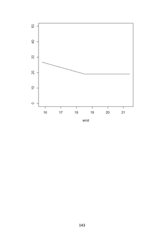
These basis functions can also be plotted, individually.
> par(mfrow = c(3, 5), # c(nrows, ncols)
+ mar = c(2, 2, 2, 2), # margin: bottom-left-top-right
+ pty = “s”)
> for (i in 2:15) {
+ j <- i – 1} # adjust index for matrices below
# Next is a 252x14 double matrix
> xp <- matrix(sapply(df[2:15], mean),
+ nrow(df),
+ ncol(df) - 1,
+ byrow = TRUE);
> colnames(xp) <- names(df[2:15])
> xr <- sapply(df, range); # 2x15 double matrix
> xp[, j] <- seq(xr[1, i], # minimum of variable i
+ xr[2, i], # maximum of variable i
+ len = nrow(df));
> xf <- predict(fatfit, xp);
> plot(xp[, j], xf,
+ xlab = names(df)[i],
+ ylab = ““,
+ ylim = c(0, 50),
+ type = “l”);](https://image.slidesharecdn.com/048d9789-800e-4318-80f7-c96b1a8df646-150122193330-conversion-gate01/85/Predictive-Analytics-using-R-173-320.jpg)


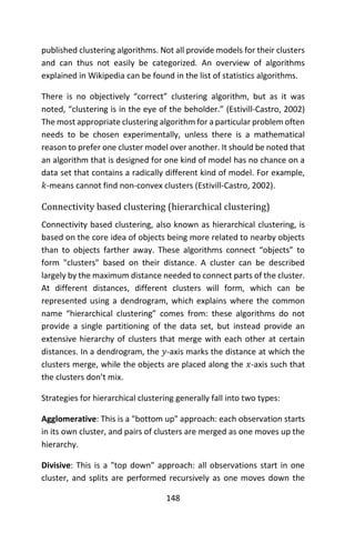


![152
Examples Using R
The ‘cluster’ package provides several useful functions for clustering
analysis. We will use one here called ‘agnes’, which performs
agglomerative hierarchical clustering of a dataset. The dataset we will
use, ‘votes.repub’ is included in the package.
## First load the package.
> library(cluster)
> data(votes.repub)
> agn1 <- agnes(votes.repub, metric = "manhattan",
+ stand = TRUE)
agn1
Call: agnes(x = votes.repub, metric = "manhattan", stand =
TRUE)
Agglomerative coefficient: 0.7977555
Order of objects:
[1] Alabama Georgia Arkansas Louisiana
Mississippi South Carolina
[7] Alaska Vermont Arizona Montana
Nevada Colorado
[13] Idaho Wyoming Utah California
Oregon Washington
[19] Minnesota Connecticut New York New Jersey
Illinois Ohio
[25] Indiana Michigan Pennsylvania New
Hampshire Wisconsin Delaware
[31] Kentucky Maryland Missouri New Mexico
West Virginia Iowa
[37] South Dakota North Dakota Kansas Nebraska
Maine Massachusetts
[43] Rhode Island Florida North Carolina Tennessee
Virginia Oklahoma
[49] Hawaii Texas
Height (summary):
Min. 1st Qu. Median Mean 3rd Qu. Max.
8.382 12.800 18.530 23.120 28.410 87.460
Available components:
[1] "order" "height" "ac" "merge" "diss"
"call" "method" "order.lab"
[9] "data"
> plot(agn1)](https://image.slidesharecdn.com/048d9789-800e-4318-80f7-c96b1a8df646-150122193330-conversion-gate01/85/Predictive-Analytics-using-R-183-320.jpg)


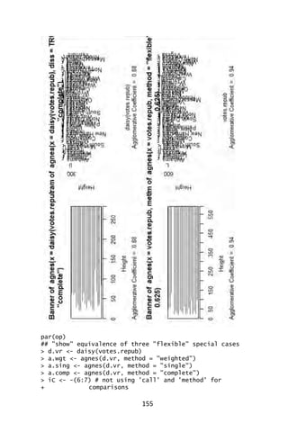
![156
> stopifnot(
+ all.equal(a.wgt [iC], agnes(d.vr, method="flexible",
+ par.method = 0.5)[iC]) ,
+ all.equal(a.sing[iC], agnes(d.vr, method="flex",
+ par.method= c(.5,.5,0, -.5))[iC]),
+ all.equal(a.comp[iC], agnes(d.vr, method="flex",
+ par.method= c(.5,.5,0, +.5))[iC]))
If you choose any height along the y-axis of the dendrogram, and move
across the dendrogram counting the number of lines that you cross, each
line represents a group that was identified when objects were joined
together into clusters. The observations in that group are represented
by the branches of the dendrogram that spread out below the line. For
example, if we look at a height of 60, and move across the 𝑥-axis at that
height, we'll cross two lines. That defines a two-cluster solution; by
following the line down through all its branches, we can see the names
of the states that are included in these two clusters. Since the 𝑦-axis
represents how close together observations were when they were
merged into clusters, clusters whose branches are very close together
(in terms of the heights at which they were merged) probably aren’t very
reliable. But if there is a big difference along the 𝑦-axis between the last
merged cluster and the currently merged one, which indicates that the
clusters formed are probably doing a good job in showing us the
structure of the data. Looking at the dendrogram for the voting data,
there are (maybe not clearly) five distinct groups at the 20-level; at the
0-level there seems to be nine distinct groups.
For this data set, it looks like either five or six groups might be an
interesting place to start investigating. This is not to imply that looking
at solutions with more clusters would be meaningless, but the data
seems to suggest that five or six clusters might be a good start. For a
problem of this size, we can see the names of the states, so we could
start interpreting the results immediately from the dendrogram, but
when there are larger numbers of observations, this won't be possible.](https://image.slidesharecdn.com/048d9789-800e-4318-80f7-c96b1a8df646-150122193330-conversion-gate01/85/Predictive-Analytics-using-R-187-320.jpg)
![157
## Exploring the dendrogram structure
> (d2 <- as.dendrogram(agn2)) # two main branches
'dendrogram' with 2 branches and 50 members total, at
height 281.9508
> d2[[1]] # the first branch
'dendrogram' with 2 branches and 8 members total, at height
116.7048
> d2[[2]] # the 2nd one { 8 + 42 = 50 }
'dendrogram' with 2 branches and 42 members total, at
height 178.4119
> d2[[1]][[1]]# first sub-branch of branch 1 .. and shorter
form
'dendrogram' with 2 branches and 6 members total, at height
72.92212
> identical(d2[[c(1,1)]], d2[[1]][[1]])
[1] TRUE
## a "textual picture" of the dendrogram :
str(d2)](https://image.slidesharecdn.com/048d9789-800e-4318-80f7-c96b1a8df646-150122193330-conversion-gate01/85/Predictive-Analytics-using-R-188-320.jpg)
![158
--[dendrogram w/ 2 branches and 50 members at h = 282]
|--[dendrogram w/ 2 branches and 8 members at h = 117]
| |--[dendrogram w/ 2 branches and 6 members at h = 72.9]
| | |--[dendrogram w/ 2 branches and 3 members at h = 60.9]
| | | |--[dendrogram w/ 2 branches and 2 members at h = 48.2]
| | | | |--leaf "Alabama"
| | | | `--leaf "Georgia"
| | | `--leaf "Louisiana"
| | `--[dendrogram w/ 2 branches and 3 members at h = 58.8]
| | |--[dendrogram w/ 2 branches and 2 members at h = 56.1]
| | | |--leaf "Arkansas"
| | | `--leaf "Florida"
| | `--leaf "Texas"
| `--[dendrogram w/ 2 branches and 2 members at h = 63.1]
| |--leaf "Mississippi"
| `--leaf "South Carolina"
`--[dendrogram w/ 2 branches and 42 members at h = 178]
|--[dendrogram w/ 2 branches and 37 members at h = 121]
| |--[dendrogram w/ 2 branches and 31 members at h = 80.5]
| | |--[dendrogram w/ 2 branches and 17 members at h = 64.5]
| | | |--[dendrogram w/ 2 branches and 13 members at h = 56.4]
| | | | |--[dendrogram w/ 2 branches and 10 members at h = 47.2]
| | | | | |--[dendrogram w/ 2 branches and 2 members at h = 28.1]
| | | | | | |--leaf "Alaska"
| | | | | | `--leaf "Michigan"
| | | | | `--[dendrogram w/ 2 branches and 8 members at h = 39.2]
| | | | | |--[dendrogram w/ 2 branches and 5 members at h = 36.8]
| | | | | | |--[dendrogram w/ 2 branches and 3 members at h = 32.9]
| | | | | | | |--[dendrogram w/ 2 branches and 2 members at h = 19.4]
| | | | | | | | |--leaf "Connecticut"
| | | | | | | | `--leaf "New York"
| | | | | | | `--leaf "New Hampshire"
| | | | | | `--[dendrogram w/ 2 branches and 2 members at h = 20.2]
| | | | | | |--leaf "Indiana"
| | | | | | `--leaf "Ohio"
| | | | | `--[dendrogram w/ 2 branches and 3 members at h = 25.3]
| | | | | |--[dendrogram w/ 2 branches and 2 members at h = 20.9]
| | | | | | |--leaf "Illinois"
| | | | | | `--leaf "New Jersey"
| | | | | `--leaf "Pennsylvania"
| | | | `--[dendrogram w/ 2 branches and 3 members at h = 42.2]
| | | | |--leaf "Minnesota"
| | | | `--[dendrogram w/ 2 branches and 2 members at h = 33.7]
| | | | |--leaf "North Dakota"
| | | | `--leaf "Wisconsin"
| | | `--[dendrogram w/ 2 branches and 4 members at h = 37.5]
| | | |--[dendrogram w/ 2 branches and 2 members at h = 26.2]
| | | | |--leaf "Iowa"
| | | | `--leaf "South Dakota"
| | | `--[dendrogram w/ 2 branches and 2 members at h = 25.9]
| | | |--leaf "Kansas"
| | | `--leaf "Nebraska"
| | `--[dendrogram w/ 2 branches and 14 members at h = 70.5]
| | |--[dendrogram w/ 2 branches and 8 members at h = 48]
| | | |--[dendrogram w/ 2 branches and 4 members at h = 43.4]
| | | | |--[dendrogram w/ 2 branches and 3 members at h = 27.8]
| | | | | |--[dendrogram w/ 2 branches and 2 members at h = 23.4]
| | | | | | |--leaf "Arizona"
| | | | | | `--leaf "Nevada"
| | | | | `--leaf "Montana"
| | | | `--leaf "Oklahoma"
| | | `--[dendrogram w/ 2 branches and 4 members at h = 43.7]
| | | |--leaf "Colorado"
| | | `--[dendrogram w/ 2 branches and 3 members at h = 31.2]
| | | |--[dendrogram w/ 2 branches and 2 members at h = 17.2]
| | | | |--leaf "Idaho"
| | | | `--leaf "Wyoming"
| | | `--leaf "Utah"
| | `--[dendrogram w/ 2 branches and 6 members at h = 54.3]
| | |--[dendrogram w/ 2 branches and 3 members at h = 33.2]
| | | |--leaf "California"
| | | `--[dendrogram w/ 2 branches and 2 members at h = 22.2]
| | | |--leaf "Oregon"
| | | `--leaf "Washington"
| | `--[dendrogram w/ 2 branches and 3 members at h = 35.1]
| | |--[dendrogram w/ 2 branches and 2 members at h = 21.1]
| | | |--leaf "Missouri"
| | | `--leaf "New Mexico"
| | `--leaf "West Virginia"
| `--[dendrogram w/ 2 branches and 6 members at h = 66.8]
| |--[dendrogram w/ 2 branches and 3 members at h = 43.4]
| | |--leaf "Delaware"
| | `--[dendrogram w/ 2 branches and 2 members at h = 33.5]
| | |--leaf "Kentucky"
| | `--leaf "Maryland"
| `--[dendrogram w/ 2 branches and 3 members at h = 30.2]
| |--[dendrogram w/ 2 branches and 2 members at h = 29.5]
| | |--leaf "North Carolina"
| | `--leaf "Tennessee"
| `--leaf "Virginia"](https://image.slidesharecdn.com/048d9789-800e-4318-80f7-c96b1a8df646-150122193330-conversion-gate01/85/Predictive-Analytics-using-R-189-320.jpg)
![159
`--[dendrogram w/ 2 branches and 5 members at h = 83.1]
|--[dendrogram w/ 2 branches and 4 members at h = 55.4]
| |--[dendrogram w/ 2 branches and 2 members at h = 32.8]
| | |--leaf "Hawaii"
| | `--leaf "Maine"
| `--[dendrogram w/ 2 branches and 2 members at h = 22.6]
| |--leaf "Massachusetts"
| `--leaf "Rhode Island"
`--leaf "Vermont"
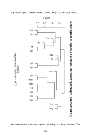
Now, we need to interpret the results of this analysis. From the
dendrogram we can see some logical clustering at the 0-level. For
instance, California, Oregon and Washington are clustered together as
we would expect. Also, at the 40-level Georgia, Alabama, Mississippi,
Arkansas, South Carolina and Louisiana are grouped together. What
other clusters make sense?
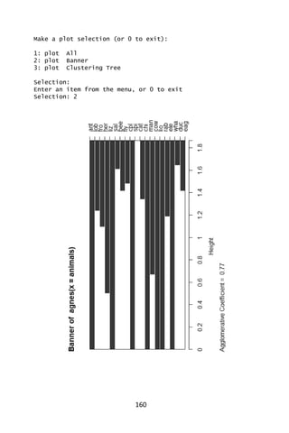
The next
plot(agnes(agriculture), ask = TRUE)
> data(animals)
> aa.a <- agnes(animals) # default method = "average"
> aa.ga <- agnes(animals, method = "gaverage")
> op <- par(mfcol=1:2, mgp=c(1.5, 0.6, 0),
+ mar=c(.1+ > c(4,3,2,1)),cex.main=0.8)
> plot(aa.a, which.plot = 2)
plot(agnes(agriculture), ask = TRUE)](https://image.slidesharecdn.com/048d9789-800e-4318-80f7-c96b1a8df646-150122193330-conversion-gate01/85/Predictive-Analytics-using-R-190-320.jpg)
![161
> plot(aa.ga, which.plot = 2)
> par(op)
## Show how "gaverage" is a "generalized average":
> aa.ga.0 <- agnes(animals, method = "gaverage",
+ par.method = 0)
> stopifnot(all.equal(aa.ga.0[iC], aa.a[iC]))](https://image.slidesharecdn.com/048d9789-800e-4318-80f7-c96b1a8df646-150122193330-conversion-gate01/85/Predictive-Analytics-using-R-192-320.jpg)

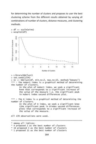
![165
* 2 proposed 15 as the best number of clusters
***** Conclusion *****
* According to the majority rule, the best number of
clusters is 3
***********************************************************
> table(nc$Best.n[1,])
0 1 2 3 11 15](https://image.slidesharecdn.com/048d9789-800e-4318-80f7-c96b1a8df646-150122193330-conversion-gate01/85/Predictive-Analytics-using-R-196-320.jpg)
![166
2 1 4 16 1 2
> barplot(table(nc$Best.n[1,]),
+ xlab="Numer of Clusters", ylab="Number of Criteria",
+ main="Number of Clusters Chosen by 26 Criteria")
> set.seed(1234)
> fit.km <- kmeans(df, 3, nstart=25)
> fit.km$size
[1] 61 68 49
> fit.km$centers
V1 V2 V3 V4 V5
V6 V7 V8
1 -1.16822514 0.8756272 -0.3037196 0.3180446 -0.6626544
0.56329925 0.87403990 0.94098462
2 0.07973544 -0.9195318 -0.3778231 -0.4643776 0.1750133 -
0.46892793 -0.07372644 0.04416309
3 1.34366784 0.1860184 0.9024258 0.2485092 0.5820616 -
0.05049296 -0.98577624 -1.23271740
V9 V10 V11 V12 V13
V14
1 -0.583942581 0.58014642 0.1667181 0.4823674 0.7648958
1.1550888
2 0.008736157 0.01821349 -0.8598525 0.4233092 0.2490794
-0.7630972
3 0.714825281 -0.74749896 0.9857177 -1.1879477 -1.2978785
-0.3789756](https://image.slidesharecdn.com/048d9789-800e-4318-80f7-c96b1a8df646-150122193330-conversion-gate01/85/Predictive-Analytics-using-R-197-320.jpg)
![167
> aggregate(wine[-1], by=list(cluster=fit.km$cluster),
mean)
cluster V2 V3 V4 V5 V6
V7 V8 V9 V10 V11
1 1 13.71148 1.997049 2.453770 17.28197 107.78689
2.842131 2.9691803 0.2891803 1.922951 5.444590
2 2 12.25412 1.914265 2.239118 20.07941 93.04412
2.248971 2.0733824 0.3629412 1.601324 3.064706
3 3 13.15163 3.344490 2.434694 21.43878 99.02041
1.678163 0.7979592 0.4508163 1.163061 7.343265
V12 V13 V14
1 1.0677049 3.154754 1110.6393
2 1.0542059 2.788529 506.5882
3 0.6859184 1.690204 627.5510
Two additional cluster plot may be useful in your analysis.
> clusplot(wine, fit.km$cluster, color=TRUE, shade=TRUE,
+ labels=2, lines=0)](https://image.slidesharecdn.com/048d9789-800e-4318-80f7-c96b1a8df646-150122193330-conversion-gate01/85/Predictive-Analytics-using-R-198-320.jpg)


![171
of these settings produces the same formulas and same results. The only
difference is the interpretation and the assumptions which have to be
imposed in order for the method to give meaningful results. The choice
of the applicable framework depends mostly on the nature of data in
hand, and on the inference task which has to be performed.
One of the lines of difference in interpretation is whether to treat the
regressors as random variables, or as predefined constants. In the first
case (random design) the regressors 𝑥𝑖 are random and sampled
together with the 𝑦𝑖 ‘s from some population, as in an observational
study. This approach allows for more natural study of the asymptotic
properties of the estimators. In the other interpretation (fixed design),
the regressors 𝑋 are treated as known constants set by a design, and 𝑦
is sampled conditionally on the values of 𝑋 as in an experiment. For
practical purposes, this distinction is often unimportant, since
estimation and inference is carried out while conditioning on 𝑋. All
results stated in this article are within the random design framework.
The primary assumption of OLS is that there is zero or negligible errors
in the independent variable, since this method only attempts to
minimize the mean squared error in the dependent variable.
Classical linear regression model
The classical model focuses on the “finite sample” estimation and
inference, meaning that the number of observations n is fixed. This
contrasts with the other approaches, which study the asymptotic
behavior of OLS, and in which the number of observations is allowed to
grow to infinity.
• Correct specification. The linear functional form is correctly
specified.
• Strict exogeneity. The errors in the regression should have
conditional mean zero (Hayashi, 2000):
𝐸[𝜀|𝑋] = 0.](https://image.slidesharecdn.com/048d9789-800e-4318-80f7-c96b1a8df646-150122193330-conversion-gate01/85/Predictive-Analytics-using-R-202-320.jpg)
![172
The immediate consequence of the exogeneity assumption is that
the errors have mean zero: 𝐸[𝜀] = 0, and that the regressors are
uncorrelated with the errors: 𝐸[𝑋′𝜀] = 0.
The exogeneity assumption is critical for the OLS theory. If it holds
then the regressor variables are called exogenous (Hayashi, 2000). If
it doesn’t, then those regressors that are correlated with the error
term are called endogenous, and then the OLS estimates become
invalid. In such case the method of instrumental variables may be
used to carry out inference.
• No linear dependence. The regressors in 𝑋 must all be linearly
independent. Mathematically it means that the matrix 𝑋 must have
full column rank almost surely (Hayashi, 2000):
𝑃𝑟[rank(𝑋) = 𝑝] = 1
Usually, it is also assumed that the regressors have finite moments
up to at least second. In such case the matrix 𝑄 𝑥𝑥 = 𝐸[𝑋′𝑋/𝑛] will
be finite and positive semi-definite. When this assumption is
violated the regressors are called linearly dependent or perfectly
multicollinear. In such case the value of the regression coefficient 𝛽
cannot be learned, although prediction of 𝑦 values is still possible for
new values of the regressors that lie in the same linearly dependent
subspace.
• Spherical errors:
𝑉𝑎𝑟[𝜀|𝑋] = 𝜎2
𝐼 𝑛
where 𝐼 𝑛 is an 𝑛 × 𝑛 identity matrix, and 𝜎2
is a parameter which
determines the variance of each observation. This 𝜎2
is considered
a nuisance parameter in the model, although usually it is also
estimated. If this assumption is violated then the OLS estimates are
still valid, but no longer efficient. It is customary to split this
assumption into two parts:](https://image.slidesharecdn.com/048d9789-800e-4318-80f7-c96b1a8df646-150122193330-conversion-gate01/85/Predictive-Analytics-using-R-203-320.jpg)
![173
• Homoscedasticity: 𝐸[𝜀𝑖
2
|𝑋] = 𝜎2
, which means that the error
term has the same variance 𝜎2
in each 𝑖 observation. When this
requirement is violated this is called heteroscedasticity, in such
case a more efficient estimator would be weighted least
squares. If the errors have infinite variance then the OLS
estimates will also have infinite variance (although by the law of
large numbers they will nonetheless tend toward the true values
so long as the errors have zero mean). In this case, robust
estimation techniques are recommended.
• Nonautocorrelation: the errors are uncorrelated between
observations: 𝐸[𝜀𝑖 𝜀𝑗|𝑋] = 0 for 𝑖 ≠ 𝑗. This assumption may be
violated in the context of time series data, panel data, cluster
samples, hierarchical data, repeated measures data,
longitudinal data, and other data with dependencies. In such
cases generalized least squares provides a better alternative
than the OLS.
• Normality. It is sometimes additionally assumed that the errors have
normal distribution conditional on the regressors (Hayashi, 2000):
𝜀|𝑋~𝒩(0, 𝜎2
𝐼 𝑛).
This assumption is not needed for the validity of the OLS method,
although certain additional finite-sample properties can be
established in case when it does (especially in the area of hypotheses
testing). Also when the errors are normal, the OLS estimator is
equivalent to the maximum likelihood estimator (MLE), and
therefore it is asymptotically efficient in the class of all regular
estimators.
Independent and identically distributed
In some applications, especially with cross-sectional data, an additional
assumption is imposed — that all observations are independent and
identically distributed (iid). This means that all observations are taken
from a random sample which makes all the assumptions listed earlier](https://image.slidesharecdn.com/048d9789-800e-4318-80f7-c96b1a8df646-150122193330-conversion-gate01/85/Predictive-Analytics-using-R-204-320.jpg)
![174
simpler and easier to interpret. Also this framework allows one to state
asymptotic results (as the sample size 𝑛 → ∞), which are understood
as a theoretical possibility of fetching new independent observations
from the data generating process. The list of assumptions in this case is:
• iid observations: (𝑥𝑖, 𝑦𝑖) is independent from, and has the same
distribution as, (𝑥𝑗, 𝑦𝑗) for all 𝑖 ≠ 𝑗;
• no perfect multicollinearity: 𝑄 𝑥𝑥 = 𝐸[𝑥𝑖 𝑥𝑗
′
]is a positive-definite
matrix;
• exogeneity: 𝐸[𝜀𝑖|𝑥𝑖] = 0
• homoscedasticity: 𝑉𝑎𝑟[𝜀𝑖|𝑥𝑖] = 𝜎2
Time series model
• The stochastic process {𝑥𝑖, 𝑦𝑖} is stationary and ergodic;
• The regressors are predetermined: 𝐸[𝑥𝑖 𝜀𝑖] = 0 for all 𝑖 = 1, … , 𝑛;
• The 𝑝 × 𝑝 matrix 𝑄 𝑥𝑥 = 𝐸[𝑥𝑖 𝑥𝑗
′
] is of full rank, and hence positive-
definite;
• {𝑥𝑖 𝜀𝑖} is a martingale difference sequence, with a finite matrix of
second moments 𝑄 𝑥𝑥𝜀2 = 𝐸[𝜀𝑖
2
𝑥𝑖 𝑥𝑗
′
]
Estimation
Suppose 𝑏 is a “candidate” value for the parameter 𝛽. The quantity 𝑦𝑖 −
𝑥𝑖
′
𝑏 is called the residual for the 𝑖-th observation, it measures the vertical
distance between the data point (𝑥𝑖, 𝑦𝑖) and the hyperplane 𝑦 = 𝑥′𝑏,
and thus assesses the degree of fit between the actual data and the
model. The sum of squared residuals (SSR) (also called the error sum of
squares (ESS) or residual sum of squares (RSS)) (Hayashi, 2000) is a
measure of the overall model fit:
𝑆(𝑏) = ∑(𝑦𝑖 − 𝑥𝑖
′
𝑏)2
𝑛
𝑖=1
= (𝑦 − 𝑋𝑏) 𝑇(𝑦 − 𝑋𝑏),
where 𝑇 denotes the matrix transpose. The value of 𝑏 which minimizes
this sum is called the OLS estimator for 𝛽. The function 𝑆(𝑏) is quadratic](https://image.slidesharecdn.com/048d9789-800e-4318-80f7-c96b1a8df646-150122193330-conversion-gate01/85/Predictive-Analytics-using-R-205-320.jpg)

![177
𝛽̂ =
∑ 𝑥𝑖 𝑦𝑖 −
1
𝑛
∑ 𝑥𝑖 ∑ 𝑦𝑖
∑ 𝑥𝑖
2
−
1
𝑛
(∑ 𝑥𝑖)2
=
Cov[𝑥, 𝑦]
Var[𝑥]
, 𝛼̂ = 𝑦̅ − 𝛽̂ 𝑥̅
Alternative derivations
In the previous section the least squares estimator 𝛽̂ was obtained as a
value that minimizes the sum of squared residuals of the model.
However it is also possible to derive the same estimator from other
approaches. In all cases the formula for OLS estimator remains the same:
𝛽̂ = (𝑋′𝑋)−1
𝑋′𝑦, the only difference is in how we interpret this result.
Geometric approach
For mathematicians, OLS is an approximate solution to an
overdetermined system of linear equations 𝑋𝛽 ≈ 𝑦, where 𝛽 is the
unknown. Assuming the system cannot be solved exactly (the number of
equations 𝑛 is much larger than the number of unknowns 𝑝), we are
looking for a solution that could provide the smallest discrepancy
between the right- and left- hand sides. In other words, we are looking
for the solution that satisfies
𝛽̂ = arg min
𝛽
‖𝑦 − 𝑋𝛽‖
where || · || is the standard 𝐿2
norm in the 𝑛-dimensional Euclidean
space 𝑅 𝑛
. The predicted quantity 𝑋𝛽 is just a certain linear combination
of the vectors of regressors. Thus, the residual vector 𝑦 − 𝑋𝛽 will have
the smallest length when 𝑦 is projected orthogonally onto the linear
subspace spanned by the columns of 𝑋. The OLS estimator in this case
can be interpreted as the coefficients of vector decomposition of 𝑦̂ =
𝑃𝑦 along the basis of 𝑋.](https://image.slidesharecdn.com/048d9789-800e-4318-80f7-c96b1a8df646-150122193330-conversion-gate01/85/Predictive-Analytics-using-R-208-320.jpg)
![179
Generalized method of moments
In iid case the OLS estimator can also be viewed as a GMM estimator
arising from the moment conditions
𝐸[𝑥𝑖(𝑦𝑖 − 𝑥𝑖
′
𝛽)] = 0.
These moment conditions state that the regressors should be
uncorrelated with the errors. Since 𝑥𝑖 is a 𝑝-vector, the number of
moment conditions is equal to the dimension of the parameter vector
𝛽, and thus the system is exactly identified. This is the so-called classical
GMM case, when the estimator does not depend on the choice of the
weighting matrix.
Note that the original strict exogeneity assumption 𝐸[𝜀𝑖|𝑥] = 0 implies
a far richer set of moment conditions than stated above. In particular,
this assumption implies that for any vector-function ƒ, the moment
condition 𝐸[ƒ(𝑥𝑖) · 𝜀𝑖] = 0 will hold. However it can be shown using the
Gauss–Markov theorem that the optimal choice of function ƒ is to take
ƒ(𝑥) = 𝑥, which results in the moment equation posted above.
Finite sample properties
First of all, under the strict exogeneity assumption the OLS estimators 𝛽̂
and 𝑠2
are unbiased, meaning that their expected values coincide with
the true values of the parameters (Hayashi, 2000):
𝐸[𝛽̂|𝑋] = 𝛽, 𝐸[𝑠2|𝑋] = 𝜎2
.
If the strict exogeneity does not hold (as is the case with many time
series models, where exogeneity is assumed only with respect to the
past shocks but not the future ones), then these estimators will be
biased in finite samples.
The variance-covariance matrix of 𝛽̂ is equal to (Hayashi, 2000)
Var[𝛽̂|𝑋] = 𝜎2(𝑋′𝑋)−1
.](https://image.slidesharecdn.com/048d9789-800e-4318-80f7-c96b1a8df646-150122193330-conversion-gate01/85/Predictive-Analytics-using-R-210-320.jpg)
![180
In particular, the standard error of each coefficient 𝛽̂𝑗 is equal to square
root of the 𝑗-th diagonal element of this matrix. The estimate of this
standard error is obtained by replacing the unknown quantity 𝜎2
with
its estimate 𝑠2
.
Thus,
𝑠𝑒̂(𝛽̂𝑗) = √ 𝑠2(𝑋′𝑋) 𝑗𝑗
−1
It can also be easily shown that the estimator is 𝛽̂ uncorrelated with the
residuals from the model (Hayashi, 2000):
Cov[𝛽̂, 𝜀̂ |𝑋] = 0.
The Gauss–Markov theorem states that under the spherical errors
assumption (that is, the errors should be uncorrelated and
homoscedastic) the estimator is efficient in the class of linear unbiased
estimators. This is called the best linear unbiased estimator (BLUE).
Efficiency should be understood as if we were to find some other
estimator 𝛽̂ which would be linear in y and unbiased, then (Hayashi,
2000)
Var[𝛽̃|𝑋] − Var[𝛽̂|𝑋]
in the sense that this is a nonnegative-definite matrix. This theorem
establishes optimality only in the class of linear unbiased estimators,
which is quite restrictive. Depending on the distribution of the error
terms 𝜀, other, non-linear estimators may provide better results than
OLS.
Assuming normality
The properties listed so far are all valid regardless of the underlying
distribution of the error terms. However if you are willing to assume that
the normality assumption holds (that is, that 𝜀~𝑁(0, 𝜎2
𝐼 𝑛)), then
additional properties of the OLS estimators can be stated.](https://image.slidesharecdn.com/048d9789-800e-4318-80f7-c96b1a8df646-150122193330-conversion-gate01/85/Predictive-Analytics-using-R-211-320.jpg)


![184
𝛽̂ 𝑐
= 𝑅(𝑅′𝑋′𝑋𝑅)−1
𝑅′
𝑋′
𝑦 + (𝐼 𝑝 − 𝑅(𝑅′
𝑋′
𝑋𝑅)−1
𝑅′𝑋′𝑋)𝑄(𝑄′𝑄)−1
𝑐,
where 𝑅 is a 𝑝 × (𝑝 − 𝑞) matrix such that the matrix [𝑄𝑅] is non-
singular, and 𝑅′𝑄 = 0. Such a matrix can always be found, although
generally it is not unique. The second formula coincides with the first in
case when 𝑋′𝑋 is invertible (Amemiya, 1985).
Large sample properties
The least squares estimators are point estimates of the linear regression
model parameters 𝛽. However, generally we also want to know how
close those estimates might be to the true values of parameters. In other
words, we want to construct the interval estimates.
Since we haven’t made any assumption about the distribution of error
term 𝜀𝑖, it is impossible to infer the distribution of the estimators 𝛽̂ and
𝜎̂2
. Nevertheless, we can apply the law of large numbers and central
limit theorem to derive their asymptotic properties as sample size n goes
to infinity. While the sample size is necessarily finite, it is customary to
assume that 𝑛 is “large enough” so that the true distribution of the OLS
estimator is close to its asymptotic limit, and the former may be
approximately replaced by the latter.
We can show that under the model assumptions, the least squares
estimator for 𝛽 is consistent (that is 𝛽̂ converges in probability to 𝛽) and
asymptotically normal:
√ 𝑛(𝛽̂ − 𝛽)
𝑑
→ 𝒩(0, 𝜎2
𝑄 𝑥𝑥
−1),
where 𝑄 𝑥𝑥 = 𝑋′𝑋.
Using this asymptotic distribution, approximate two-sided confidence
intervals for the 𝑗-th component of the vector 𝛽̂ can be constructed as
at the 1 − 𝛼 confidence level,](https://image.slidesharecdn.com/048d9789-800e-4318-80f7-c96b1a8df646-150122193330-conversion-gate01/85/Predictive-Analytics-using-R-215-320.jpg)
![185
𝛽𝑗 ∈ [𝛽̂𝑗 ± 𝑞1−𝛼 2⁄
𝒩(0,1)
√
1
𝑛
𝜎̂2[𝑄 𝑥𝑥
−1] 𝑗𝑗]
where 𝑞 denotes the quantile function of standard normal distribution,
and [·] 𝑗𝑗 is the 𝑗-th diagonal element of a matrix.
Similarly, the least squares estimator for 𝜎2
is also consistent and
asymptotically normal (provided that the fourth moment of 𝜀𝑖 exists)
with limiting distribution
√ 𝑛(𝜎̂2
− 𝜎2)
𝑑
→ 𝒩(0, 𝐸[𝜀𝑖
4
] − 𝜎4
).
These asymptotic distributions can be used for prediction, testing
hypotheses, constructing other estimators, etc. As an example consider
the problem of prediction. Suppose 𝑥0 is some point within the domain
of distribution of the regressors, and one wants to know what the
response variable would have been at that point. The mean response is
the quantity 𝒚0 = 𝒙0
′
𝜷, whereas the predicted response is 𝒚̂0 = 𝒙0
′
𝜷̂.
Clearly the predicted response is a random variable, its distribution can
be derived from that of :
√ 𝑛(𝑦̂0 − 𝑦0)
𝑑
→ 𝒩(0, 𝜎2
𝑥0
′
𝑄 𝑥𝑥
−1
𝑥0),
which allows construct confidence intervals for mean response 𝑦0 to be
constructed:
𝑦0 ∈ [𝑥0
′
𝛽̂ ± 𝑞1−𝛼 2⁄
𝒩(0,1)
√
1
𝑛
𝜎̂2 𝑥0
′
𝑄 𝑥𝑥
−1 𝑥0]
at the 1 − 𝛼 confidence level.
Example with real data
This example exhibits the common mistake of ignoring the condition of
having zero error in the dependent variable.](https://image.slidesharecdn.com/048d9789-800e-4318-80f7-c96b1a8df646-150122193330-conversion-gate01/85/Predictive-Analytics-using-R-216-320.jpg)

![188
estimate: (
1
𝑛
𝜎̂2[𝑄 𝑥𝑥
−1] 𝑗𝑗)
1 2⁄
• The 𝑡-statistic and 𝑝-value columns are testing whether any of the
coefficients might be equal to zero. The 𝑡-statistic is calculated
simply as 𝑡 = 𝛽̂𝑗 𝜎̂𝑗⁄ . If the errors ε follow a normal distribution, 𝑡
follows a Student-t distribution. Under weaker conditions, 𝑡 is
asymptotically normal. Large values of 𝑡 indicate that the null
hypothesis can be rejected and that the corresponding coefficient is
not zero. The second column, p-value, expresses the results of the
hypothesis test as a significance level. Conventionally, 𝑝-values
smaller than 0.05 are taken as evidence that the population
coefficient is nonzero.
• 𝑅-squared𝑅2
is the coefficient of determination indicating
goodness-of-fit of the regression. This statistic will be equal to one if
fit is perfect, and to zero when regressors 𝑋 have no explanatory
power whatsoever. This is a biased estimate of the population R-
squared, and will never decrease if additional regressors are added,
even if they are irrelevant.
• Adjusted 𝑅-squared𝑅2
is a slightly modified version of 𝑅2
, designed
to penalize for the excess number of regressors which do not add to
the explanatory power of the regression. This statistic is always
smaller than 𝑅2
𝑅2
, can decrease as new regressors are added, and
even be negative for poorly fitting models:
𝑅̅2
= 1 −
𝑛 − 1
𝑛 − 𝑝
(1 − 𝑅2)
• Log-likelihood is calculated under the assumption that errors follow
normal distribution. Even though the assumption is not very
reasonable, this statistic may still find its use in conducting LR tests.
• Durbin–Watson statistic tests whether there is any evidence of serial
correlation between the residuals. As a rule of thumb, the value
smaller than 2 will be an evidence of positive correlation.
• Akaike information criterion and Schwarz criterion are both used for
model selection. Generally when comparing two alternative models,
smaller values of one of these criteria will indicate a better model](https://image.slidesharecdn.com/048d9789-800e-4318-80f7-c96b1a8df646-150122193330-conversion-gate01/85/Predictive-Analytics-using-R-219-320.jpg)


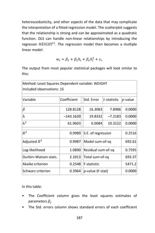
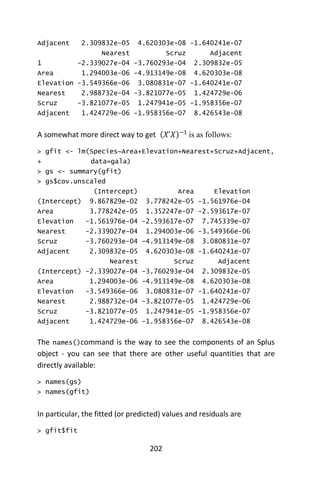
![195
Species The number of species of tortoise found on the island
Endemics The number of endemic species
Elevation The highest elevation of the island (m)
Nearest The distance from the nearest island (km)
Scruz The distance from Santa Cruz island
(km)
Adjacent The area of the adjacent island (km2)
The data were presented by Johnson and Raven (Johnson & Raven,
1973) and also appear in Weisberg (Weisberg, 2005). We have filled in
some missing values for simplicity. Fitting a linear model in R is done
using the lm() command. Notice the syntax for specifying the predictors
in the model. This is the so-called Wilkinson-Rogers notation. In this
case, since all the variables are in the gala data frame, we must use the
data= argument.
First, we generate a series of plots of various species-area relations. We
consider three models: Linear, Gleason, and log-Arrhenius.
1. Linear model: 𝑆~Normal(𝜇, 𝜎2
) with identity link such that 𝜇 = 𝛽0 +
𝛽1 𝐴.
2. Gleason model: 𝑆~Normal(𝜇, 𝜎2
) with identity link such that 𝜇 =
𝛽0 + 𝛽1log𝐴.
3. log-Arrhenius model: 𝑆~Normal(𝜇, 𝜎2
) with identity link such that
𝜇 = 𝛽0 𝐴 𝛽1.
Model 1 is a Linear Model. We fit a linear model on the original scale,
model 1 above and obtain the log-likelihood (with logLik) and the AIC
(with AIC).
> model1<-lm(Species~Area,data=gala)
> logLik(model1)
‘log Lik.’ -177.0993 (df=3)
> AIC(model1)
[1] 360.1985
We superimpose the fitted model on a scatter plot of the data.
> plot(gala$Area,gala$Species, xlab=‘Area’, ylab=‘Species’)](https://image.slidesharecdn.com/048d9789-800e-4318-80f7-c96b1a8df646-150122193330-conversion-gate01/85/Predictive-Analytics-using-R-226-320.jpg)
![196
> abline(model1,col=2, lty=2)
> mtext(‘Model 1: linear model’, side=3, line=.5)
Model 2 is a Gleason Model. The Gleason model requires a log-
transformed predictor, but an untransformed response.
> model2<-lm(Species~log(Area),data=gala)
> logLik(model2)
‘log Lik.’ -169.9574 (df=3)
> AIC(model2)
[1] 345.9147
> plot(log(gala$Area), gala$Species, xlab=‘log(Area)’,
+ ylab=‘Species’)
> abline(model2,col=2,lty=2)
> mtext( ‘Model 2: Gleason model‘, side=3, line=.5)](https://image.slidesharecdn.com/048d9789-800e-4318-80f7-c96b1a8df646-150122193330-conversion-gate01/85/Predictive-Analytics-using-R-227-320.jpg)
![197
Model 3 is a log-Arrhenius. The log-Arrhenius model is just an ordinary
regression model in which both the response and predictor are log-
transformed.
> model3<-lm(log(Species)~log(Area), data=gala)
> logLik(model3)
‘log Lik.’ -34.23973 (df=3)
> AIC(model3)
[1] 74.47946
> plot(log(gala$Area), log(gala$Species), xlab=‘log(Area)’,
+ ylab=‘log(Species)’)
> abline(model3,col=2,lty=2)
> mtext(‘Model 3: log-Arrhenius model‘, side=3, line=.5)](https://image.slidesharecdn.com/048d9789-800e-4318-80f7-c96b1a8df646-150122193330-conversion-gate01/85/Predictive-Analytics-using-R-228-320.jpg)

![199
# n is the sample size
> AIC.func<-function(LL,K,n,modelnames)
+ {
+ AIC<- -2*LL + 2*K
+ AICc<-AIC + 2*K*(K+1)/(n-K-1)
+ output<-cbind(LL,K,AIC,AICc)
+ colnames(output)<-c(‘LogL’,’K’,’AIC’,’AICc’)
+ minAICc<-min(output[,”AICc”])
+ deltai<-output[,”AICc”]-minAICc
+ rel.like<-exp(-deltai/2)
+ wi<-round(rel.like/sum(rel.like),3)
+ out<-data.frame(modelnames,output,deltai,wi)
+ out
+ }
> AIC.func(loglike,numparms,dim(gala)[1],model.names)
modelnames LogL K AIC AICc deltai wi
1 Linear -177.09927 3 360.19853 361.12161 285.7191 0
2 Gleason -169.95737 3 345.91473 346.83781 271.4353 0
3 Log-Arrhenius -34.23973 3 74.47946 75.40253 0.0000 1
Based on the output we see there is only one model that has any
empirical support, the log-Arrhenius model. For reasons we will not
explain here, although the log-Arrhenius model fits well, it is not
guaranteed to be optimal. For the Galapagos data, a model that allows
there to be heteroscedasticity on the scale of the original response is to
be preferred.
The previous models only examine the Species-Area relationship. We
now consider additional variables: Endemics, Elevation, Nearest,
Scruz, and Adjacent. We will call our model gfit.
> gfit <- lm(Species~Area + Elevation + Nearest + Scruz +
+ Adjacent, data=gala)
> summary(gfit)
Call:
> lm(formula = Species~Area + Elevation + Nearest + Scruz +
+ Adjacent, data=gala)
> summary(gfit)](https://image.slidesharecdn.com/048d9789-800e-4318-80f7-c96b1a8df646-150122193330-conversion-gate01/85/Predictive-Analytics-using-R-230-320.jpg)
![200
Call:
lm(formula = Species ~ Area + Elevation + Nearest + Scruz +
Adjacent,
data = gala)
Residuals:
Min 1Q Median 3Q Max
-111.679 -34.898 -7.862 33.460 182.584
Coefficients:
Estimate Std. Error t value Pr(>|t|)
(Intercept) 7.068221 19.154198 0.369 0.715351
Area -0.023938 0.022422 -1.068 0.296318
Elevation 0.319465 0.053663 5.953 3.82e-06 ***
Nearest 0.009144 1.054136 0.009 0.993151
Scruz -0.240524 0.215402 -1.117 0.275208
Adjacent -0.074805 0.017700 -4.226 0.000297 ***
---
Signif. codes: 0 ‘***’ 0.001 ‘**’ 0.01 ‘*’ 0.05 ‘.’ 0.1 ‘ ‘
1
Residual standard error: 60.98 on 24 degrees of freedom
Multiple R-squared: 0.7658, Adjusted R-squared: 0.7171
F-statistic: 15.7 on 5 and 24 DF, p-value: 6.838e-07
We can identify several useful quantities in this output. Other statistical
packages tend to produce output quite similar to this. One useful feature
of R is that it is possible to directly calculate quantities of interest. Of
course, it is not necessary here because the lm() function does the job
but it is very useful when the statistic you want is not part of the pre-
packaged functions.
First we make the 𝑋-matrix
> x <- cbind(1,gala[,-c(1,2)])
and here’s the response 𝑦:
> y <- gala$Species](https://image.slidesharecdn.com/048d9789-800e-4318-80f7-c96b1a8df646-150122193330-conversion-gate01/85/Predictive-Analytics-using-R-231-320.jpg)

![203
Baltra Bartolome Caldwell Champion
116.7259460 -7.2731544 29.3306594 10.3642660
Coamano Daphne.Major Daphne.Minor Darwin
-36.3839155 43.0877052 33.9196678 -9.0189919
Eden Enderby Espanola Fernandina
28.3142017 30.7859425 47.6564865 96.9895982
Gardner1 Gardner2 Genovesa Isabela
-4.0332759 64.6337956 -0.4971756 386.4035578
Marchena Onslow Pinta Pinzon
88.6945404 4.0372328 215.6794862 150.4753750
Las.Plazas Rabida SanCristobal SanSalvador
35.0758066 75.5531221 206.9518779 277.6763183
SantaCruz SantaFe SantaMaria Seymour
261.4164131 85.3764857 195.6166286 49.8050946
Tortuga Wolf
52.9357316 26.7005735
> gfit$res
Baltra Bartolome Caldwell Champion
-58.725946 38.273154 -26.330659 14.635734
Coamano Daphne.Major Daphne.Minor Darwin
38.383916 -25.087705 -9.919668 19.018992
Eden Enderby Espanola Fernandina
-20.314202 -28.785943 49.343513 -3.989598
Gardner1 Gardner2 Genovesa Isabela
62.033276 -59.633796 40.497176 -39.403558
Marchena Onslow Pinta Pinzon
-37.694540 -2.037233 -111.679486 -42.475375
Las.Plazas Rabida SanCristobal SanSalvador
-23.075807 -5.553122 73.048122 -40.676318
SantaCruz SantaFe SantaMaria Seymour
182.583587 -23.376486 89.383371 -5.805095
Tortuga Wolf
-36.935732 -5.700573
We can get 𝛽̂directly:
> xtxi %*% t(x) %*% y
[,1]
1 7.068220709](https://image.slidesharecdn.com/048d9789-800e-4318-80f7-c96b1a8df646-150122193330-conversion-gate01/85/Predictive-Analytics-using-R-234-320.jpg)
![204
Area -0.023938338
Elevation 0.319464761
Nearest 0.009143961
Scruz -0.240524230
Adjacent -0.074804832
or in a computationally efficient and stable manner:
> solve(t(x) %*% x, t(x) %*% y)
[,1]
[1,] 7.068220709
[2,] -0.023938338
[3,] 0.319464761
[4,] 0.009143961
[5,] -0.240524230
[6,] -0.074804832
We can estimate 𝜎using the estimator in the text:
> root1<-sum((gfit$res)^2)
> sqrt(root1/(30-6))
[1] 60.97519
Compare this to the results above (Residual standard error).
We may also obtain the standard errors for the coefficients. Also diag()
returns the diagonal of a matrix):
> sqrt(diag(xtxi))*60.97519
1 Area Elevation Nearest
19.15419834 0.02242235 0.05366281 1.05413598
Scruz Adjacent
0.21540225 0.01770019
Finally we may compute 𝑅2
:
> 1-sum((gfit$res)ˆ2)/sum((y-mean(y))ˆ2)
[1] 0.7658469](https://image.slidesharecdn.com/048d9789-800e-4318-80f7-c96b1a8df646-150122193330-conversion-gate01/85/Predictive-Analytics-using-R-235-320.jpg)


![210
𝑏(𝜇) = 𝜃 = 𝑿𝜷, which allows 𝑿 𝑇
Y to be a sufficient statistic for
𝜷.
Following is a table of several exponential-family distributions in
common use and the data they are typically used for, along with the
canonical link functions and their inverses (sometimes referred to as the
mean function, as done here).
Common distributions with typical uses and canonical link functions
Distribution Supportofdistribution Typicaluses Link
name
Linkfunction Meanfunction
Normal real:(−∞, ∞) Linear-responsedata Identity 𝑿𝜷 = 𝜇 𝜇 = 𝑿𝜷
Exponentialreal:(0, ∞) Exponential-response
data,scaleparameters
Inverse 𝑿𝜷 = −𝜇−1
𝜇 = (−𝑿𝜷)−1
Gamma
Inverse
Gaussian
real:(0, ∞) Inverse
squared
𝑿𝜷 = −𝜇−2 𝜇
= (−𝑿𝜷)−1 2⁄
Poisson integer:(0, ∞) countofoccurrencesin
fixedamountof
time/space
Log 𝑿𝜷 = ln(𝜇) 𝜇 = 𝑒 𝑿𝜷
Bernoulli integer:[0,1] outcomeofsingleyes/no
occurrence
Logit 𝑿𝜷
= ln (
𝜇
1 − 𝜇
)
𝜇 =
1
1 + 𝑒 𝑿𝜷
Binomial integer:[0, 𝑁] countof#of“yes”
occurrencesoutofN
yes/nooccurrences
Categorical integer:[0, 𝐾] outcomeofsingleK-way
occurrenceK-vectorofinteger:
[0,1],whereexactly
oneelementinthe
vectorhasthe
value1
MultinomialK-vectorof[0, 𝑁] countofoccurrencesof
differenttypes(1..K)out
ofNtotalK-way
occurrences
In the cases of the exponential and gamma distributions, the domain of
the canonical link function is not the same as the permitted range of the
mean. In particular, the linear predictor may be negative, which would
give an impossible negative mean. When maximizing the likelihood,
precautions must be taken to avoid this. An alternative is to use a](https://image.slidesharecdn.com/048d9789-800e-4318-80f7-c96b1a8df646-150122193330-conversion-gate01/85/Predictive-Analytics-using-R-241-320.jpg)
![211
noncanonical link function.
Note also that in the case of the Bernoulli, binomial, categorical and
multinomial distributions, the support of the distributions is not the
same type of data as the parameter being predicted. In all of these cases,
the predicted parameter is one or more probabilities, i.e. real numbers
in the range [0,1]. The resulting model is known as logistic regression (or
multinomial logistic regression in the case that 𝐾-way rather than binary
values are being predicted).
For the Bernoulli and binomial distributions, the parameter is a single
probability, indicating the likelihood of occurrence of a single event. The
Bernoulli still satisfies the basic condition of the generalized linear model
in that, even though a single outcome will always be either 0 or 1, the
expected value will nonetheless be a real-valued probability, i.e. the
probability of occurrence of a “yes” (or 1) outcome. Similarly, in a
binomial distribution, the expected value is 𝑁𝑝, i.e. the expected
proportion of “yes” outcomes will be the probability to be predicted.
For categorical and multinomial distributions, the parameter to be
predicted is a 𝐾-vector of probabilities, with the further restriction that
all probabilities must add up to 1. Each probability indicates the
likelihood of occurrence of one of the 𝐾 possible values. For the
multinomial distribution, and for the vector form of the categorical
distribution, the expected values of the elements of the vector can be
related to the predicted probabilities similarly to the binomial and
Bernoulli distributions.
Fitting
Maximum likelihood
The maximum likelihood estimates can be found using an iteratively
reweighted least squares algorithm using either a Newton–Raphson
method with updates of the form:
𝜷(𝑡+1)
= 𝜷(𝑡)
+ 𝒥−1
(𝜷(𝑡)
)𝑢(𝜷(𝑡)
),](https://image.slidesharecdn.com/048d9789-800e-4318-80f7-c96b1a8df646-150122193330-conversion-gate01/85/Predictive-Analytics-using-R-242-320.jpg)
![213
to suppose that the distribution function is the normal distribution with
constant variance and the link function is the identity, which is the
canonical link if the variance is known.
For the normal distribution, the generalized linear model has a closed
form expression for the maximum-likelihood estimates, which is
convenient. Most other GLMs lack closed form estimates.
Binomial data
When the response data, Y, are binary (taking on only values 0 and 1),
the distribution function is generally chosen to be the Bernoulli
distribution and the interpretation of 𝜇𝑖 is then the probability, 𝑝, of 𝑌𝑖
taking on the value one.
There are several popular link functions for binomial functions; the most
typical is the canonical logit link:
𝑔(𝑝) = ln (
𝑝
1 − 𝑝
).
GLMs with this setup are logistic regression models (or logit models).
In addition, the inverse of any continuous cumulative distribution
function (CDF) can be used for the link since the CDF‘s range is [0,1], the
range of the binomial mean. The normal CDF Φ is a popular choice and
yields the probit model. Its link is
𝑔(𝑝) = Φ−1(𝑝).
The reason for the use of the probit model is that a constant scaling of
the input variable to a normal CDF (which can be absorbed through
equivalent scaling of all of the parameters) yields a function that is
practically identical to the logit function, but probit models are more
tractable in some situations than logit models. (In a Bayesian setting in
which normally distributed prior distributions are placed on the
parameters, the relationship between the normal priors and the normal
CDF link function means that a probit model can be computed using](https://image.slidesharecdn.com/048d9789-800e-4318-80f7-c96b1a8df646-150122193330-conversion-gate01/85/Predictive-Analytics-using-R-244-320.jpg)
![214
Gibbs sampling, while a logit model generally cannot.)
The complementary log-log function log(−log(1 − 𝑝)) may also be
used. This link function is asymmetric and will often produce different
results from the probit and logit link functions.
The identity link is also sometimes used for binomial data to yield the
linear probability model, but a drawback of this model is that the
predicted probabilities can be greater than one or less than zero. In
implementation it is possible to fix the nonsensical probabilities outside
of [0,1], but interpreting the coefficients can be difficult. The model’s
primary merit is that near 𝑝 = 0.5 it is approximately a linear
transformation of the probit and logit―econometricians sometimes call
this the Harvard model.
The variance function for binomial data is given by:
Var(𝑌𝑖) = 𝜏𝜇𝑖(1 − 𝜇𝑖),
where the dispersion parameter 𝜏 is typically fixed at exactly one. When
it is not, the resulting quasi-likelihood model often described as binomial
with overdispersion or quasi-binomial.
Multinomial regression
The binomial case may be easily extended to allow for a multinomial
distribution as the response (also, a Generalized Linear Model for
counts, with a constrained total). There are two ways in which this is
usually done:
Ordered response
If the response variable is an ordinal measurement, then one may fit a
model function of the form:
𝑔(𝜇 𝑚) = 𝜂 𝑚 = 𝛽0 + 𝑋1 𝛽1 + ⋯ + 𝑋 𝑝 𝛽 𝑝 + 𝛾2 + ⋯ + 𝛾 𝑚
= 𝜂1 + 𝛾2 + ⋯ + 𝛾 𝑚,
where 𝜇 𝑚 = 𝑃(𝑌 ≤ 𝑚), for 𝑚 > 2. Different links 𝑔 lead to](https://image.slidesharecdn.com/048d9789-800e-4318-80f7-c96b1a8df646-150122193330-conversion-gate01/85/Predictive-Analytics-using-R-245-320.jpg)


![220
NOTE you can use the column headers as variable names if you specify
the data-frame using “data=“
> fitB1
Call: glm(formula = cbind(status, 1 - status) ~ rx, family
= binomial,
data = rats)
Coefficients:
(Intercept) rx
-1.450 1.127
Degrees of Freedom: 149 Total (i.e. Null); 148 Residual
Null Deviance: 174
Residual Deviance: 165.3 AIC: 169.3
> summary(fitB1)$coef
Estimate Std. Error z value Pr(>|z|)
(Intercept) -1.450010 0.2549063 -5.688404 1.282324e-08
rx 1.127237 0.3835089 2.939272 3.289845e-03
Coefficients fitted by MLE, link=“logit“ is default for binomial-family
data: this is logistic regression.
The standard error is found as sqrt of diagonal in variance:
> sqrt(diag(summary(fitB1)$cov.scaled))
(Intercept) rx
0.2549063 0.3835089
“Deviance” = “Residual Deviance” = -2*logLik
> c(fitB1$deviance, -2*logLik(fitB1))
[1] 165.2738 165.2738
“Null.deviance” is -2 times the logLik for the same model with only a
constant term
> c(fitB1$null.dev,](https://image.slidesharecdn.com/048d9789-800e-4318-80f7-c96b1a8df646-150122193330-conversion-gate01/85/Predictive-Analytics-using-R-251-320.jpg)
![221
+ -2*logLik(update(fitB1, formula = .~ 1))
+ )
[1] 173.9746 173.9746
NOTE the use of the “update” function to refit a model of the same type
as the one previously done: in the model formula, the left-hand side
term is a “.” to indicate that it is the same as before. We have changed
the right-hand side from rx (which automatically included intercept
along with rx predictor) to one with “1” or intercept alone.
Next use “update” to change the fitB1 model not in its model formula
but in its specified link within the binomial “family”.
> fitB2 = update(fitB1, family=binomial(link=“probit”))
> rbind(logit= fitB1$coef, probit= fitB2$coef,
+ rescal.probit = fitB2$coef/0.5513)
(Intercept) rx
logit -1.4500102 1.1272368
probit -0.8778963 0.6760028
rescal.probit -1.5924112 1.2261977
Recall that we use deviance and differences between them because
Wilks’ Theorem says that 2 times the difference between logLik for a
model with 𝑝 extra parameter dimensions versus logLik for a base
model is equal to approximately a chi-square (𝑝, df) variate when the
base model is the true one (see Chapter 10).
Model Quality
LET’s use this idea to examine the quality of the model with predictor
log(time) in the model along with rx.
NOTE that we must put the expression log(time) within I( ) to have it
evaluated and constructed as a new predictor within the glm fitting
function.
> fitB3 = update(fitB1, formula= . ~ . + I(log(time)))
The “data” is the same now as in fitB1, so “time” is the column in the](https://image.slidesharecdn.com/048d9789-800e-4318-80f7-c96b1a8df646-150122193330-conversion-gate01/85/Predictive-Analytics-using-R-252-320.jpg)
![222
data-frame, and a log(time) predictor is created under “glm”
It is reasonable to use “time” as a predictor, because the range of times
is not too different for rats who generate tumors, so “time” is not really
a response variable.
> summary(rats$time[rats$status==1])
Min. 1st Qu. Median Mean 3rd Qu. Max.
34.00 66.75 80.00 77.28 92.50 104.00
> summary(rats$time[rats$status==0])
Min. 1st Qu. Median Mean 3rd Qu. Max.
45.00 83.50 104.00 93.85 104.00 104.00
> cbind(rats[1:10,], model.matrix(fitB3)[1:10,])
litter rx time status (Intercept) rx I(log(time))
1 1 1 101 0 1 1 4.615121
2 1 0 49 1 1 0 3.891820
3 1 0 104 0 1 0 4.644391
4 2 1 104 0 1 1 4.644391
5 2 0 102 0 1 0 4.624973
6 2 0 104 0 1 0 4.644391
7 3 1 104 0 1 1 4.644391
8 3 0 104 0 1 0 4.644391
9 3 0 104 0 1 0 4.644391
10 4 1 77 0 1 1 4.343805
The first 4 columns are the original “rats” data. The last 3 are the design
matrix columns created by glm. So we can look at the new model fit for
significance of coefficients:
> summary(fitB3)$coef
Estimate Std. Error z value Pr(>|z|)
(Intercept) 17.868661 4.4924813 3.977459 6.965559e-05
rx 1.194019 0.4284626 2.786751 5.323935e-03
I(log(time)) -4.355407 1.0180848 -4.278040 1.885462e-05
Or alternatvely compare deviances or logLik’s with fitB1
> c(2*(logLik(fitB3)-logLik(fitB1)), fitB1$dev-fitB3$dev)](https://image.slidesharecdn.com/048d9789-800e-4318-80f7-c96b1a8df646-150122193330-conversion-gate01/85/Predictive-Analytics-using-R-253-320.jpg)
![223
[1] 24.37307 24.37307
This is LRT stat to be compared with chisq 1 df.
> 1-pchisq(24.373,1)
[1] 7.937339e-07
This is still highly significant but somewhat different p-value from the
I(log(time)) coef probably because the model is still far from the
right one.
We could try to enter additional terms like log(time)^2 or rx *
log(time)
> fitB4 = update(fitB3, .~. + I(rx*log(time)) +
+ I(log(time)^2))
> summary(fitB4)$coef
Estimate Std. Error z value
(Intercept) -9.784968 52.690740 -0.1857056
rx -13.501206 8.732837 -1.5460274
I(log(time)) 10.179730 24.364938 0.4178024
I(rx * log(time)) 3.324780 1.973389 1.6848069
I(log(time)^2) -1.871215 2.819823 -0.6635932
Pr(>|z|)
(Intercept) 0.85267560
rx 0.12209794
I(log(time)) 0.67609159
I(rx * log(time)) 0.09202582
I(log(time)^2) 0.50695069
This time, the new variables do NOT look significant which we can check
also through deviances:
> fitB3$dev - fitB4$dev
[1] 3.901065
This result is to be compared with chisq 2df, so it is not at all significant.
We can also do these deviance comparisons all at once by looking at an
“analysis of deviance” table](https://image.slidesharecdn.com/048d9789-800e-4318-80f7-c96b1a8df646-150122193330-conversion-gate01/85/Predictive-Analytics-using-R-254-320.jpg)
![224
> anova(fitB4)
Analysis of Deviance Table
Model: binomial, link: logit
Response: cbind(status, 1 - status)
Terms added sequentially (first to last)
Df Deviance Resid. Df Resid. Dev
NULL 149 173.97
rx 1 8.7008 148 165.27
I(log(time)) 1 24.3731 147 140.90
I(rx * log(time)) 1 3.4784 146 137.42
I(log(time)^2) 1 0.4226 145 137.00
As in an ANOVA table, in which RSS replaced Deviance these “Deviance
values” are the amounts by which the current model-fitting line
decreases the deviance: (recall that fitB1 uses rx only, fitB3 augments
by log(time), and fitB4 by log(time) plus the 2 additional
rx*log(tim) and log(time)^2 terms.
> Devs = c(fitB1$null.dev, fitB1$dev, fitB3$dev,
+ update(fitB3, .~.+I(rx*log(time)))$dev,
+ fitB4$dev)
> Devs
[1] 173.9746 165.2738 140.9007 137.4223 136.9997
> round (-diff(Devs), 3 )### successive differences of llks
[1] 8.701 24.373 3.478 0.423 ### give Deviance col
in “anova”](https://image.slidesharecdn.com/048d9789-800e-4318-80f7-c96b1a8df646-150122193330-conversion-gate01/85/Predictive-Analytics-using-R-255-320.jpg)


![241
coefficients to be matched for each possible value of the discrete
variable. (In a case like this, only three of the four dummy variables are
independent of each other, in the sense that once the values of three of
the variables are known, the fourth is automatically determined. Thus,
it is only necessary to encode three of the four possibilities as dummy
variables. This also means that when all four possibilities are encoded,
the overall model is not identifiable in the absence of additional
constraints such as a regularization constraint. Theoretically, this could
cause problems, but in reality almost all logistic regression models are
fit with regularization constraints.)
Outcome variables
Formally, the outcomes 𝑌𝑖 are described as being Bernoulli-distributed
data, where each outcome is determined by an unobserved probability
𝑝𝑖 that is specific to the outcome at hand, but related to the explanatory
variables. This can be expressed in any of the following equivalent forms:
𝑌𝑖|𝑥1,𝑖, … , 𝑥 𝑚,𝑖~Bernoulli(𝑝𝑖)
𝐸[𝑌𝑖|𝑥1,𝑖, … , 𝑥 𝑚,𝑖] = 𝑝𝑖
Pr(𝑌𝑖 = 𝑦𝑖|𝑥1,𝑖, … , 𝑥 𝑚,𝑖) = {
𝑝𝑖 if 𝑦𝑖 = 1
1 − 𝑝𝑖 if 𝑦𝑖 = 0
Pr(𝑌𝑖 = 𝑦𝑖|𝑥1,𝑖, … , 𝑥 𝑚,𝑖) = 𝑝𝑖
𝑦𝑖
(1 − 𝑝𝑖)(1−𝑦𝑖)
The meanings of these four lines are:
1. The first line expresses the probability distribution of each 𝑌𝑖:
Conditioned on the explanatory variables, it follows a Bernoulli
distribution with parameters 𝑝𝑖, the probability of the outcome of 1 for
trial 𝑖. As noted above, each separate trial has its own probability of
success, just as each trial has its own explanatory variables. The
probability of success 𝑝𝑖 is not observed, only the outcome of an
individual Bernoulli trial using that probability.
2. The second line expresses the fact that the expected value of each 𝑌𝑖
is equal to the probability of success 𝑝𝑖, which is a general property of
the Bernoulli distribution. In other words, if we run a large number of](https://image.slidesharecdn.com/048d9789-800e-4318-80f7-c96b1a8df646-150122193330-conversion-gate01/85/Predictive-Analytics-using-R-272-320.jpg)

![243
• The resulting explanatory variables 𝑥0,𝑖, 𝑥1,𝑖, … , 𝑥 𝑚,𝑖 are then
grouped into a single vector 𝑿𝑖 of size 𝑚 +1.
This makes it possible to write the linear predictor function as follows:
𝒇(𝑖) = 𝜷 ∙ 𝑿𝑖,
using the notation for a dot product between two vectors.
As a generalized linear model
The particular model used by logistic regression, which distinguishes it
from standard linear regression and from other types of regression
analysis used for binary-valued outcomes, is the way the probability of a
particular outcome is linked to the linear predictor function:
logit(𝐸[𝑌𝑖|𝑥1,𝑖, … , 𝑥 𝑚,𝑖]) = logit(𝑝𝑖)
= ln (
𝑝𝑖
1 − 𝑝𝑖
) = 𝛽1 𝑥1,𝑖 + 𝛽2 𝑥1,𝑖 + ⋯ + 𝛽 𝑚 𝑥 𝑚,𝑖
Written using the more compact notation described above, this is:
logit(𝐸[𝑌𝑖|𝑿𝑖]) = logit(𝑝𝑖) = ln (
𝑝𝑖
1 − 𝑝𝑖
) = 𝜷 ∙ 𝑿𝑖.
This formulation expresses logistic regression as a type of generalized
linear model, which predicts variables with various types of probability
distributions by fitting a linear predictor function of the above form to
some sort of arbitrary transformation of the expected value of the
variable.
The intuition for transforming using the logit function (the natural log of
the odds) was explained above. It also has the practical effect of
converting the probability (which is bounded to be between 0 and 1) to
a variable that ranges over (−∞, +∞) — thereby matching the potential
range of the linear prediction function on the right side of the equation.
Note that both the probabilities 𝑝𝑖 and the regression coefficients are
unobserved, and the means of determining them is not part of the model](https://image.slidesharecdn.com/048d9789-800e-4318-80f7-c96b1a8df646-150122193330-conversion-gate01/85/Predictive-Analytics-using-R-274-320.jpg)
![244
itself. They are typically determined by some sort of optimization
procedure, e.g. maximum likelihood estimation, which finds values that
best fit the observed data (i.e. that give the most accurate predictions
for the data already observed), usually subject to regularization
conditions that seek to exclude unlikely values, e.g. extremely large
values for any of the regression coefficients. The use of a regularization
condition is equivalent to doing maximum a posteriori (MAP) estimation,
an extension of maximum likelihood. (Regularization is most commonly
done using a squared regularizing function, which is equivalent to
placing a zero-mean Gaussian prior distribution on the coefficients, but
other regularizers are also possible.) Whether or not regularization is
used, it is usually not possible to find a closed-form solution; instead, an
iterative numerical method must be used, such as iteratively reweighted
least squares (IRLS) or, more commonly these days, a quasi-Newton
method such as the L-BFGS method.
The interpretation of the 𝛽𝑗 parameter estimates is as the additive effect
on the log of the odds for a unit change in the 𝑗th explanatory variable.
In the case of a dichotomous explanatory variable, for instance gender,
𝑒 𝛽
is the estimate of the odds of having the outcome for, say, males
compared with females.
An equivalent formula uses the inverse of the logit function, which is the
logistic function, i.e.:
𝐸[𝑌𝑖|𝑿𝑖] = 𝑝𝑖 = (𝜷 ∙ 𝑿𝑖) =
1
1 + 𝑒−𝜷∙𝑿𝑖
.
The formula can also be written (somewhat awkwardly) as a probability
distribution (specifically, using a probability mass function):
Pr(𝑌𝑖 = 𝑦𝑖|𝑿𝑖) = 𝑝𝑖
𝑦𝑖
(1 − 𝑝𝑖)(1−𝑦𝑖)
= (
1
1 + 𝑒−𝜷∙𝑿𝑖
)
𝑦𝑖
(1 −
1
1 + 𝑒−𝜷∙𝑿𝑖
)
1−𝑦𝑖
.](https://image.slidesharecdn.com/048d9789-800e-4318-80f7-c96b1a8df646-150122193330-conversion-gate01/85/Predictive-Analytics-using-R-275-320.jpg)


![254
An example of this distribution is the fraction of seeds (𝑝𝑖) that
germinate after 𝑛𝑖 are planted. In terms of expected values, this model
is expressed as follows:
𝑝𝑖 = 𝐸 [
𝑌𝑖
𝑛𝑖
| 𝑿𝑖],
so that
logit (𝐸 [
𝑌𝑖
𝑛𝑖
| 𝑿𝑖]) = logit(𝑝𝑖) = ln (
𝑝𝑖
1 − 𝑝𝑖
) = 𝜷 ∙ 𝑿𝑖,
Or equivalently:
Pr(𝑌𝑖 = 𝑦𝑖|𝑿𝒊) = (
𝑛𝑖
𝑘𝑖
) 𝑝𝑖
𝑦𝑖
(1 − 𝑝𝑖) 𝑛 𝑖−𝑦𝑖
= (
𝑛𝑖
𝑘𝑖
) (
1
1 + 𝑒−𝜷∙𝑿𝑖
)
𝑦𝑖
(1 −
1
1 + 𝑒−𝜷∙𝑿𝑖
)
1−𝑦𝑖
.
This model can be fit using the same sorts of methods as the above more
basic model.
Bayesian logistic regression
In a Bayesian statistics context, prior distributions are normally placed
on the regression coefficients, usually in the form of Gaussian
distributions. Unfortunately, the Gaussian distribution is not the
conjugate prior of the likelihood function in logistic regression; in fact,
the likelihood function is not an exponential family and thus does not
have a conjugate prior at all. As a result, the posterior distribution is
difficult to calculate, even using standard simulation algorithms (e.g.
Gibbs sampling).
There are various possibilities:
• Don’t do a proper Bayesian analysis, but simply compute a maximum
a posteriori point estimate of the parameters. This is common, for
example, in “maximum entropy” classifiers in machine learning.
• Use a more general approximation method such as the Metropolis–](https://image.slidesharecdn.com/048d9789-800e-4318-80f7-c96b1a8df646-150122193330-conversion-gate01/85/Predictive-Analytics-using-R-285-320.jpg)

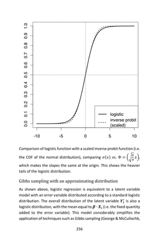

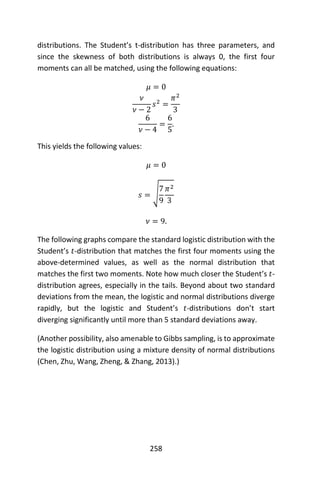
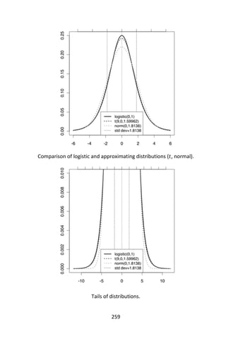
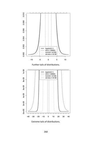


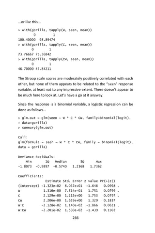
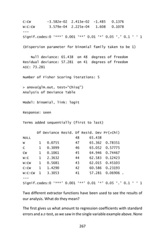
![268
of the coefficients are significantly different from zero (but a few are
close). The deviance was reduced by 8.157 points on 7 degrees of
freedom, for a p-value of...
> 1 - pchisq(8.157, df=7)
[1] 0.3189537
Overall, the model appears to have performed poorly, showing no
significant reduction in deviance (no significant difference from the null
model).
The second print out shows the same overall reduction in deviance, from
65.438 to 57.281 on 7 degrees of freedom. In this print out, however,
the reduction in deviance is shown for each term, added sequentially
first to last. Of note is the three-way interaction term, which produced a
nearly significant reduction in deviance of 3.305 on 1 degree of freedom
(p = 0.069).
In the event you are encouraged by any of this, the following graph might
be revealing...
> plot(glm.out$fitted)
> abline(v=30.5,col=“red”)
> abline(h=.3,col=“green”)
> abline(h=.5,col=“green”)
> text(15,.9,”seen = 0”)
> text(40,.9,”seen = 1”)](https://image.slidesharecdn.com/048d9789-800e-4318-80f7-c96b1a8df646-150122193330-conversion-gate01/85/Predictive-Analytics-using-R-299-320.jpg)
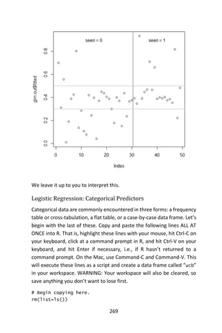
![270
gender = rep(c(“female”,”male”),c(1835,2691))
admitted =
rep(c(“yes”,”no”,”yes”,”no”),c(557,1278,1198,1493))
dept =
rep(c(“A”,”B”,”C”,”D”,”E”,”F”,”A”,”B”,”C”,”D”,”E”,”F”),
c(89,17,202,131,94,24,19,8,391,244,299,317))
dept2 =
rep(c(“A”,”B”,”C”,”D”,”E”,”F”,”A”,”B”,”C”,”D”,”E”,”F”),
c(512,353,120,138,53,22,313,207,205,279,138,351))
department = c(dept,dept2)
ucb = data.frame(gender,admitted,department)
rm(gender,admitted,dept,dept2,department)
ls()
# End copying here.
[1] “ucb”
Data sets that are purely categorical are not economically represented
in case-by-case data frames, and so the built-in data sets that are purely
categorical come in the form of tables (contingency tables or
crosstabulations). We have just taken the data from one of these (the
“UCBAdmissions” built-in data set) and turned it into a case-by-case
data frame. It’s the classic University of California, Berkeley, admissions
data from 1973 describing admissions into six different graduate
programs broken down by gender. Let’s examine the “UCBAdmissions”
data set.
> ftable(UCBAdmissions, col.vars=“Admit”)
Admit Admitted Rejected
Gender Dept
Male A 512 313
B 353 207
C 120 205
D 138 279
E 53 138
F 22 351
Female A 89 19
B 17 8
C 202 391](https://image.slidesharecdn.com/048d9789-800e-4318-80f7-c96b1a8df646-150122193330-conversion-gate01/85/Predictive-Analytics-using-R-301-320.jpg)
![271
D 131 244
E 94 299
F 24 317
The data are from 1973 and show admissions by gender to the top six
grad programs at the University of California, Berkeley. Looked at as a
two-way table, there appears to be a bias against admitting women...
> dimnames(UCBAdmissions)
$Admit
[1] “Admitted” “Rejected”
$Gender
[1] “Male” “Female”
$Dept
[1] “A” “B” “C” “D” “E” “F”
> margin.table(UCBAdmissions, c(2,1))
Admit
Gender Admitted Rejected
Male 1198 1493
Female 557 1278
However, there are also relationships between “Gender” and “Dept” as
well as between “Dept” and “Admit”, which means the above
relationship may be confounded by “Dept” (or “Dept” might be a
lurking variable, in the language of traditional regression analysis).
Perhaps a logistic regression with the binomial variable “Admit” as the
response can tease these variables apart.
If there is a way to conveniently get that flat table into a data frame
(without splitting an infinitive), I do not know it. So I had to do this...
> ucb.df =
+ data.frame(gender=rep(c(“Male”,”Female”),c(6,6)),
+ dept=rep(LETTERS[1:6],2),
+ yes=c(512,353,120,138,53,22,89,17,202,131,94,24),
+ no=c(313,207,205,279,138,351,19,8,391,244,299,317))](https://image.slidesharecdn.com/048d9789-800e-4318-80f7-c96b1a8df646-150122193330-conversion-gate01/85/Predictive-Analytics-using-R-302-320.jpg)

![273
Df Deviance Resid. Df Resid. Dev Pr(>Chi)
NULL 11 877.06
gender 1 93.45 10 783.61 < 2.2e-16
dept 5 763.40 5 20.20 < 2.2e-16
gender:dept 5 20.20 0 0.00 0.001144
This is a saturated model, meaning we have used up all our degrees of
freedom, and there is no residual deviance left over at the end.
Saturated models always fit the data perfectly. In this case, it appears
the saturated model is required to explain the data adequately. If we
leave off the interaction term, for example, we will be left with a residual
deviance of 20.2 on 5 degrees of freedom, and the model will be rejected
(𝑝 = 0.001144). It appears all three terms are making a significant
contribution to the model.
How they are contributing appears if we use the other extractor...
> summary(glm.out)
Call:
glm(formula = mod.form, family = binomial(logit), data =
ucb.df)
Deviance Residuals:
[1] 0 0 0 0 0 0 0 0 0 0 0 0
Coefficients:
Estimate Std. Error z value Pr(>|z|)
(Intercept) 1.5442 0.2527 6.110 9.94e-10
genderMale -1.0521 0.2627 -4.005 6.21e-05
deptB -0.7904 0.4977 -1.588 0.11224
deptC -2.2046 0.2672 -8.252 < 2e-16
deptD -2.1662 0.2750 -7.878 3.32e-15
deptE -2.7013 0.2790 -9.682 < 2e-16
deptF -4.1250 0.3297 -12.512 < 2e-16
genderMale:deptB 0.8321 0.5104 1.630 0.10306
genderMale:deptC 1.1770 0.2996 3.929 8.53e-05](https://image.slidesharecdn.com/048d9789-800e-4318-80f7-c96b1a8df646-150122193330-conversion-gate01/85/Predictive-Analytics-using-R-304-320.jpg)
![274
genderMale:deptD 0.9701 0.3026 3.206 0.00135
genderMale:deptE 1.2523 0.3303 3.791 0.00015
genderMale:deptF 0.8632 0.4027 2.144 0.03206
(Dispersion parameter for binomial family taken to be 1)
Null deviance: 8.7706e+02 on 11 degrees of freedom
Residual deviance: -1.6676e-13 on 0 degrees of freedom
AIC: 92.94
Number of Fisher Scoring iterations: 3
These are the regression coefficients for each predictor in the model,
with the base level of each factor being suppressed. Remember, we are
predicting log odd”...
> exp(-1.0521) # antilog of the genderMale coefficient
[1] 0.3492037
> 1/exp(-1.0521)
[1] 2.863658
This shows that men were actually at a significant disadvantage when
department and the interaction are controlled. The odds of a male being
admitted were only 0.35 times the odds of a female being admitted. The
reciprocal of this turns it on its head. All else being equal, the odds of
female being admitted were 2.86 times the odds of a male being
admitted.
Each coefficient compares the corresponding predictor to the base level.
So...
> exp(-2.2046)
[1] 0.1102946
...the odds of being admitted to department C were only about 1/9th the
odds of being admitted to department A, all else being equal. If you want
to compare, for example, department C to department D, do this...
> exp(-2.2046) / exp(-2.1662) # C:A / D:A leaves C:D](https://image.slidesharecdn.com/048d9789-800e-4318-80f7-c96b1a8df646-150122193330-conversion-gate01/85/Predictive-Analytics-using-R-305-320.jpg)
![275
[1] 0.9623279
All else equal, the odds of being admitted to department C were 0.96
times the odds of being admitted to department D. (To be honest, I am
not sure I am comfortable with the interaction in this model. You might
want to examine the interaction, and if you think it doesn’t merit
inclusion, run the model again without it. Statistics are nice, but in the
end it’s what makes sense that should rule the day.)](https://image.slidesharecdn.com/048d9789-800e-4318-80f7-c96b1a8df646-150122193330-conversion-gate01/85/Predictive-Analytics-using-R-306-320.jpg)


![286
From these plots, we can identify observations 9, 25, and 51as possibly
problematic to our model. We can look at these observations to see
which states they represent.
> cdata[c(9, 25, 51), 1:2]
sid state
9 9 fl
25 25 ms
51 51 dc
DC, Florida and Mississippi have either high leverage or large residuals.
We can display the observations that have relatively large values of
Cook’s D. A conventional cut-off point is (frac{4}{n}), where n is the
number of observations in the data set. We will use this criterion to](https://image.slidesharecdn.com/048d9789-800e-4318-80f7-c96b1a8df646-150122193330-conversion-gate01/85/Predictive-Analytics-using-R-317-320.jpg)
![287
select the values to display.
> library(MASS)
> d1 <- cooks.distance(ols)
> r <- stdres(ols)
> a <- cbind(cdata, d1, r)
> a[d1 > 4/51, ]
sid state crime murder pctmetro pctwhite pcths poverty
1 1 ak 761 9.0 41.8 75.2 86.6 9.1
9 9 fl 1206 8.9 93.0 83.5 74.4 17.8
25 25 ms 434 13.5 30.7 63.3 64.3 24.7
51 51 dc 2922 78.5 100.0 31.8 73.1 26.4
single d1 r
1 14.3 0.1254750 -1.397418
9 10.6 0.1425891 2.902663
25 14.7 0.6138721 -3.562990
51 22.1 2.6362519 2.616447
We probably should drop DC to begin with since it is not even a state.
We include it in the analysis just to show that it has large Cook’s D and
demonstrate how it will be handled by rlm. Now we will look at the
residuals. We will generate a new variable called absr1, which is the
absolute value of the residuals (because the sign of the residual doesn’t
matter). We then print the ten observations with the highest absolute
residual values.
> rabs <- abs(r)
> a <- cbind(cdata, d1, r, rabs)
> asorted <- a[order(-rabs), ]
> asorted[1:10, ]
sid state crime murder pctmetro pctwhite pcths poverty
25 25 ms 434 13.5 30.7 63.3 64.3 24.7
9 9 fl 1206 8.9 93.0 83.5 74.4 17.8
51 51 dc 2922 78.5 100.0 31.8 73.1 26.4
46 46 vt 114 3.6 27.0 98.4 80.8 10.0
26 26 mt 178 3.0 24.0 92.6 81.0 14.9
21 21 me 126 1.6 35.7 98.5 78.8 10.7
1 1 ak 761 9.0 41.8 75.2 86.6 9.1
31 31 nj 627 5.3 100.0 80.8 76.7 10.9](https://image.slidesharecdn.com/048d9789-800e-4318-80f7-c96b1a8df646-150122193330-conversion-gate01/85/Predictive-Analytics-using-R-318-320.jpg)

![289
> hweights2 <- hweights[order(rr.huber$w), ]
> hweights2[1:15, ]
state resid weight
25 ms -846.08536 0.2889618
9 fl 679.94327 0.3595480
46 vt -410.48310 0.5955740
51 dc 376.34468 0.6494131
26 mt -356.13760 0.6864625
21 me -337.09622 0.7252263
31 nj 331.11603 0.7383578
14 il 319.10036 0.7661169
1 ak -313.15532 0.7807432
20 md 307.19142 0.7958154
19 ma 291.20817 0.8395172
18 la -266.95752 0.9159411
2 al 105.40319 1.0000000
3 ar 30.53589 1.0000000
4 az -43.25299 1.0000000
We can see that roughly, as the absolute residual goes down, the weight
goes up. In other words, cases with a large residuals tend to be down-
weighted. This output shows us that the observation for Mississippi will
be down-weighted the most. Florida will also be substantially down-
weighted. All observations not shown above have a weight of 1. In OLS
regression, all cases have a weight of 1. Hence, the more cases in the
robust regression that have a weight close to one, the closer the results
of the OLS and robust regressions.
Next, let’s run the same model, but using the bisquare weighting
function. Again, we can look at the weights.
> rr.bisquare <- rlm(crime ~ poverty + single, data =
+ cdata, psi = psi.bisquare)
> summary(rr.bisquare)
Call: rlm(formula = crime ~ poverty + single, data = cdata,
psi = psi.bisquare)
Residuals:
Min 1Q Median 3Q Max](https://image.slidesharecdn.com/048d9789-800e-4318-80f7-c96b1a8df646-150122193330-conversion-gate01/85/Predictive-Analytics-using-R-320-320.jpg)
![290
-905.59 -140.97 -14.98 114.65 668.38
Coefficients:
Value Std. Error t value
(Intercept) -1535.3338 164.5062 -9.3330
poverty 11.6903 7.8987 1.4800
single 175.9303 17.0678 10.3077
Residual standard error: 202.3 on 48 degrees of freedom
> biweights <- data.frame(state = cdata$state, resid =
+ rr.bisquare$resid, weight = rr.bisquare$w)
> biweights2 <- biweights[order(rr.bisquare$w), ]
> biweights2[1:15, ]
state resid weight
25 ms -905.5931 0.007652565
9 fl 668.3844 0.252870542
46 vt -402.8031 0.671495418
26 mt -360.8997 0.731136908
31 nj 345.9780 0.751347695
18 la -332.6527 0.768938330
21 me -328.6143 0.774103322
1 ak -325.8519 0.777662383
14 il 313.1466 0.793658594
20 md 308.7737 0.799065530
19 ma 297.6068 0.812596833
51 dc 260.6489 0.854441716
50 wy -234.1952 0.881660897
5 ca 201.4407 0.911713981
10 ga -186.5799 0.924033113
We can see that the weight given to Mississippi is dramatically lower
using the bisquare weighting function than the Huber weighting function
and the parameter estimates from these two different weighting
methods differ. When comparing the results of a regular OLS regression
and a robust regression, if the results are very different, you will most
likely want to use the results from the robust regression. Large
differences suggest that the model parameters are being highly
influenced by outliers. Different functions have advantages and](https://image.slidesharecdn.com/048d9789-800e-4318-80f7-c96b1a8df646-150122193330-conversion-gate01/85/Predictive-Analytics-using-R-321-320.jpg)


![300
Use 𝑈 instead of 𝑋 for classification. The examples that are not
prototypes are called “absorbed” points.
It is efficient to scan the training examples in order of decreasing border
ratio (Mirkes, 2011).
The border ratio of a training example 𝑥 is defined as
𝑎(𝑥) = ‖𝑥′
− 𝑦‖ ‖𝑥 − 𝑦‖⁄
where ‖𝑥 − 𝑦‖ is the distance to the closest example 𝑦 having a
different color than x, and ‖𝑥′
− 𝑦‖is the distance from y to its closest
example 𝑥′ with the same label as 𝑥.
The border ratio is in the interval [0,1] because ‖𝑥′
− 𝑦‖ never exceeds
‖𝑥 − 𝑦‖. This ordering gives preference to the borders of the classes for
inclusion in the set of prototypes 𝑈. A point of a different label than x is
called external to 𝑥. The calculation of the border ratio is illustrated by
the figure on the right. The data points are labeled by colors: the initial
point is 𝑥 and its label is red. External points are blue and green. The
closest to x external point is 𝑦. The closest to y red point is 𝑥′. The border
ratio 𝑎(𝑥) = ‖𝑥′
− 𝑦‖ ‖𝑥 − 𝑦‖⁄ is the attribute of the initial point 𝑥.
Calculation of the border ratio.
Three types of points: prototypes, class-outliers, and absorbed points.](https://image.slidesharecdn.com/048d9789-800e-4318-80f7-c96b1a8df646-150122193330-conversion-gate01/85/Predictive-Analytics-using-R-331-320.jpg)


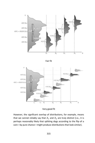


![323
design-based inference that is standard in finite-population survey
sampling.
Derived linear model
Kempthorne uses the randomization-distribution and the assumption of
unit-treatment additivity to produce a derived linear model, very similar
to the textbook model discussed previously (Hinkelmann & Kempthorne,
2008).] The test statistics of this derived linear model are closely
approximated by the test statistics of an appropriate normal linear
model, according to approximation theorems and simulation studies
(Hinkelmann & Kempthorne, 2008). However, there are differences. For
example, the randomization-based analysis results in a small but
(strictly) negative correlation between the observations (Bailey, 2008)
(Hinkelmann & Kempthorne, 2008). In the randomization-based
analysis, there is no assumption of a normal distribution and certainly no
assumption of independence. On the contrary, the observations are
dependent.
The randomization-based analysis has the disadvantage that its
exposition involves tedious algebra and extensive time. Since the
randomization-based analysis is complicated and is closely
approximated by the approach using a normal linear model, most
teachers emphasize the normal linear model approach. Few statisticians
object to model-based analysis of balanced randomized experiments.
Statistical models for observational data
However, when applied to data from non-randomized experiments or
observational studies, model-based analysis lacks the warrant of
randomization (Kempthorne, 1979). For observational data, the
derivation of confidence intervals must use subjective models, as
emphasized by Ronald A. Fisher and his followers. In practice, the
estimates of treatment-effects from observational studies generally are
often inconsistent. In practice, “statistical models” and observational
data are useful for suggesting hypotheses that should be treated very
cautiously by the public (Freedman, 2005).](https://image.slidesharecdn.com/048d9789-800e-4318-80f7-c96b1a8df646-150122193330-conversion-gate01/85/Predictive-Analytics-using-R-354-320.jpg)
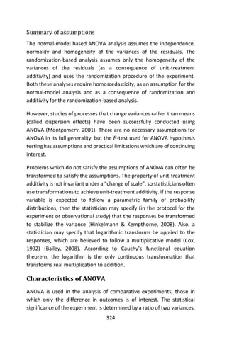


![327
of which produce the same result:
• The textbook method is to compare the observed value of 𝐹 with
the critical value of F determined from tables. The critical value of 𝐹
is a function of the degrees of freedom of the numerator and the
denominator and the significance level (𝛼). If 𝐹 ≥ 𝐹Critical, the null
hypothesis is rejected.
• The computer method calculates the probability (𝑝-value) of a value
of F greater than or equal to the observed value. The null hypothesis
is rejected if this probability is less than or equal to the significance
level (𝛼).
The ANOVA 𝐹-test is known to be nearly optimal in the sense of
minimizing false negative errors for a fixed rate of false positive errors
(i.e. maximizing power for a fixed significance level). For example, to test
the hypothesis that various medical treatments have exactly the same
effect, the 𝐹-test’s 𝑝-values closely approximate the permutation test’s
𝑝-values: The approximation is particularly close when the design is
balanced (Hinkelmann & Kempthorne, 2008). Such permutation tests
characterize tests with maximum power against all alternative
hypotheses, as observed by Rosenbaum (Rosenbaum, 2002). The
ANOVA 𝐹–test (of the null-hypothesis that all treatments have exactly
the same effect) is recommended as a practical test, because of its
robustness against many alternative distributions (Moore & McCabe,
2003).
Extended logic
ANOVA consists of separable parts; partitioning sources of variance and
hypothesis testing can be used individually. ANOVA is used to support
other statistical tools. Regression is first used to fit more complex models
to data, then ANOVA is used to compare models with the objective of
selecting simple(r) models that adequately describe the data. “Such
models could be fit without any reference to ANOVA, but ANOVA tools
could then be used to make some sense of the fitted models, and to test
hypotheses about batches of coefficients.” (Gelman, 2005) “[W]e think](https://image.slidesharecdn.com/048d9789-800e-4318-80f7-c96b1a8df646-150122193330-conversion-gate01/85/Predictive-Analytics-using-R-358-320.jpg)


![336
Now we combine them into one long vector, with a second vector,
group, identifying group membership:
> y = c(y1, y2, y3)
> n = rep(7, 3)
> n
[1] 7 7 7
> group = rep(1:3, n)
> group
[1] 1 1 1 1 1 1 1 2 2 2 2 2 2 2 3 3 3 3 3 3 3
Here are summaries by group and for the combined data. First we show
stem-leaf diagrams.
> tmp = tapply(y, group, stem)
The decimal point is at the |
16 | 8
17 | 6
18 | 28
19 | 17
20 | 1
The decimal point is at the |
15 | 9
16 | 4
17 | 47
18 | 47
19 | 1
The decimal point is at the |
15 | 29
16 | 57
17 | 17](https://image.slidesharecdn.com/048d9789-800e-4318-80f7-c96b1a8df646-150122193330-conversion-gate01/85/Predictive-Analytics-using-R-367-320.jpg)

![338
> anova(fit)
Analysis of Variance Table
Response: y
Df Sum Sq Mean Sq F value Pr(>F)
group 2 11.007 5.5033 3.9683 0.03735 *
Residuals 18 24.963 1.3868
---
Signif. codes: 0 ‘***’ 0.001 ‘**’ 0.01 ‘*’ 0.05 ‘.’ 0.1 ‘
‘ 1
The anova(fit) object can be used for other computations on the
handout and in class. For instance, the tabled F values can be found by
the following. First we extract the treatment and error degrees of
freedom. Then we use qt to get the tabled 𝐹 values.
> df = anova(fit)[, “Df”]
> names(df) = c(“trt”, “err”)
> df
trt err
2 18
> alpha = c(0.05, 0.01)
> qf(alpha, df[“trt”], df[“err”], lower.tail = FALSE)
[1] 3.554557 6.012905
A confidence interval on the pooled variance can be computed as well
using the anova(fit) object. First we get the residual sum of squares,
SSTrt, then we divide by the appropriate chi-square tabled values.
> anova(fit)[“Residuals”, “Sum Sq”]
[1] 24.96286
> anova(fit)[“Residuals”, “Sum Sq”]/qchisq(c(0.025, 0.975),
18)
[1] 3.0328790 0.7918086
anova(fit)[“Residuals”, “Sum Sq”]/qchisq(c(0.025, 0.975),
18,lower.tail = FALSE)
[1] 0.7918086 3.0328790](https://image.slidesharecdn.com/048d9789-800e-4318-80f7-c96b1a8df646-150122193330-conversion-gate01/85/Predictive-Analytics-using-R-369-320.jpg)


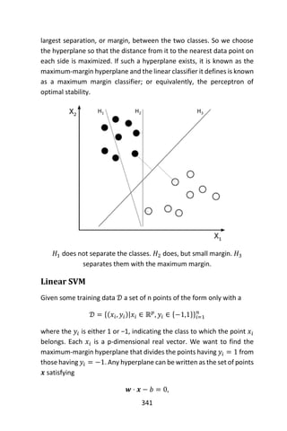
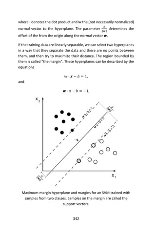

![344
arg min
(𝒘,𝑏)
1
2
‖𝒘‖2
,
subject to (for any 𝑖 = 1, … , 𝑛)
𝑦𝑖(𝒘 ⋅ 𝒙𝑖 − 𝑏) ≥ 1.
By introducing Lagrange multipliers 𝜶, the previous constrained problem
can be expressed as
arg min
𝒘,𝑏
max
𝜶≥0
{
1
2
‖𝑤‖2
− ∑ 𝜶𝑖[𝑦𝑖(𝒘 ⋅ 𝒙𝑖 − 𝑏) − 1]
𝑛
𝑖=1
},
that is, we look for a saddle point. In doing so all the points which can be
separated as 𝑦𝑖(𝒘 ⋅ 𝒙𝑖 − 𝑏) > 1 do not matter since we must set the
corresponding 𝜶𝑖 to zero.
This problem can now be solved by standard quadratic programming
techniques and programs. The “stationary” Karush–Kuhn–Tucker
condition implies that the solution can be expressed as a linear
combination of the training vectors
𝒘 = ∑ 𝛼𝑖 𝑦𝑖 𝒙𝑖
𝑛
𝑖=1
.
Only a few 𝛼𝑖 will be greater than zero. The corresponding 𝒙𝒊 are exactly
the support vectors, which lie on the margin and satisfy
𝑦𝑖(𝒘 ⋅ 𝒙𝑖 − 𝑏) = 1. From this one can derive that the support vectors
also satisfy
𝒘 ⋅ 𝒙𝑖 − 𝑏 = 1 𝑦𝑖 = 𝑦𝑖 ⟺ 𝑏 = 𝒘 ⋅ 𝒙𝒊 − 𝑦𝑖⁄ ,
which allows one to define the offset b. In practice, it is more robust to
average over all support vectors:
𝑏 =
1
𝑁𝑆𝑉
∑(𝒘 ⋅ 𝒙𝒊 − 𝑦𝑖).
𝑁 𝑆𝑉
𝑖=1](https://image.slidesharecdn.com/048d9789-800e-4318-80f7-c96b1a8df646-150122193330-conversion-gate01/85/Predictive-Analytics-using-R-375-320.jpg)

![346
∑ 𝛼𝑖 𝑦𝑖 = 0
𝑛
𝑖=1
.
Soft margin
In 1995, Corinna Cortes and Vladimir N. Vapnik suggested a modified
maximum margin idea that allows for mislabeled examples (Cortes &
Vapnik, 1995). If there exists no hyperplane that can split the “yes” and
“no” examples, the Soft Margin method will choose a hyperplane that
splits the examples as cleanly as possible, while still maximizing the
distance to the nearest cleanly split examples. The method introduces
non-negative slack variables, 𝜉𝑖, which measure the degree of
misclassification of the data 𝑥𝑖
𝑦𝑖(𝒘 ⋅ 𝒙𝑖 − 𝑏) ≥ 1 − 𝜉𝑖, 1 ≤ 𝑖 ≤ 𝑛. (2)
The objective function is then increased by a function which penalizes
non-zero 𝜉𝑖, and the optimization becomes a trade-off between a large
margin and a small error penalty. If the penalty function is linear, the
optimization problem becomes:
arg min
𝒘,𝜉,𝑏
{
1
2
‖𝒘‖2
+ 𝐶 ∑ 𝜉𝑖
𝑛
𝑖=1
},
subject to (for any 𝑖 = 1, … , 𝑛)
𝑦𝑖(𝒘 ⋅ 𝒙𝑖 − 𝑏) ≥ 1 − 𝜉𝑖, 𝜉𝑖 ≥ 0.
This constraint along with the objective of minimizing ‖𝒘‖ can be solved
using Lagrange multipliers as done above. One has then to solve the
following problem:
arg min
𝒘,𝜉,𝑏
max
𝜶,𝜷
{
1
2
‖𝒘‖2
+ 𝐶 ∑ 𝜉𝑖
𝑛
𝑖=1
− ∑ 𝛼𝑖[𝑦𝑖(𝒘 ⋅ 𝒙𝒊 − 𝑏) − 1 + 𝜉𝑖] − ∑ 𝛽𝑖 𝜉𝑖
𝑛
𝑖=1
𝑛
𝑖=1
},](https://image.slidesharecdn.com/048d9789-800e-4318-80f7-c96b1a8df646-150122193330-conversion-gate01/85/Predictive-Analytics-using-R-377-320.jpg)


![351
also treat partially labeled data in semi-supervised learning by following
the principles of transduction (Joachims, 1999). Here, in addition to the
training set 𝒟, the learner is also given a set
𝒟∗
= {𝒙𝑖
∗
|𝒙𝑖
∗
∈ ℝ 𝑝}𝑖=1
𝑘
of test examples to be classified. Formally, a transductive support vector
machine is defined by the following primal optimization problem:[2]
Minimize (in 𝒘, 𝑏, 𝒚∗
)
1
2
‖𝒘‖ 𝟐
subject to (for any 𝑖 = 1, … , 𝑛 and any𝑗 = 1, … , 𝑘)
𝑦𝑖(𝒘 ⋅ 𝒙𝑖 − 𝑏) ≥ 1,
𝑦𝑗
∗
(𝒘 ⋅ 𝒙𝒋
∗
− 𝑏) ≥ 1,
and
𝑦𝑗
∗
∈ {−1,1}.
Transductive support vector machines were introduced by Vladimir N.
Vapnik in 1998.
Structured SVM
SVMs have been generalized to structured SVMs, where the label space
is structured and of possibly infinite size.
Regression
A version of SVM for regression was proposed in 1996 by Vladimir N.
Vapnik, Harris Drucker, Christopher J. C. Burges, Linda Kaufman and
Alexander J. Smola (Drucker, Burges, Kaufman, Smola, & Vapnik, 1996).
This method is called support vector regression (SVR). The model
produced by support vector classification (as described above) depends
only on a subset of the training data, because the cost function for](https://image.slidesharecdn.com/048d9789-800e-4318-80f7-c96b1a8df646-150122193330-conversion-gate01/85/Predictive-Analytics-using-R-382-320.jpg)
![353
used in the kernel trick.
The special case of linear support vector machines can be solved more
efficiently by the same kind of algorithms used to optimize its close
cousin, logistic regression; this class of algorithms includes sub-gradient
descent (e.g., PEGASOS (Shalev-Shwartz, Singer, & Srebro, 2007)) and
coordinate descent (e.g., LIBLINEAR (Fan, Chang, Hsieh, Wang, & C.J.,
2008)). The general kernel SVMs can also be solved more efficiently
using sub-gradient descent (e.g. P-packSVM (Zhu, Chen, Wang, Zhu, &
Chen, 2009)), especially when parallelization is allowed.
Kernel SVMs are available in many machine learning toolkits, including
LIBSVM, MATLAB, SVMlight, scikit-learn, Shogun, Weka, Shark [8],
JKernelMachines [9] and others.
Applications
SVMs can be used to solve various real world problems:
• SVMs are helpful in text and hypertext categorization as their
application can significantly reduce the need for labeled training
instances in both the standard inductive and transductive settings.
• Classification of images can also be performed using SVMs.
Experimental results show that SVMs achieve significantly higher
search accuracy than traditional query refinement schemes after
just three to four rounds of relevance feedback.
• SVMs are also useful in medical science to classify proteins with up
to 90% of the compounds classified correctly.
• Hand-written characters can be recognized using SVM
Software
Software for SVM modeling include Gini-SVM in Octave, kernlab in R,
SVMlight, SPSS Modeler, and MATLAB.](https://image.slidesharecdn.com/048d9789-800e-4318-80f7-c96b1a8df646-150122193330-conversion-gate01/85/Predictive-Analytics-using-R-384-320.jpg)


![356
Support Vector Machine object of class “ksvm”
SV type: C-bsvc (classification)
parameter : cost C = 10
Gaussian Radial Basis kernel function.
Hyperparameter : sigma = 0.1
Number of Support Vectors : 32
Objective Function Value : -5.8442 -3.0652 -136.9786
Training error : 0.02
Probability model included.
> predict(irismodel, iris[c(3, 10, 56, 68, 107, 120), -5]
+ , type = “probabilities”)
setosa versicolor virginica
[1,] 0.985040508 0.007941886 0.007017606
[2,] 0.981634222 0.010962854 0.007402924
[3,] 0.004004929 0.970726183 0.025268888
[4,] 0.007777874 0.990465191 0.001756935
[5,] 0.012370962 0.103044282 0.884584756
[6,] 0.010869688 0.205778364 0.783351948
> predict(irismodel, iris[c(3, 10, 56, 68, 107, 120), -5]
+ , type = “decision”)
[,1] [,2] [,3]
[1,] -1.460398 -1.1910251 -3.8868836
[2,] -1.357355 -1.1749491 -4.2107843
[3,] 1.647272 0.7655001 -1.3205306
[4,] 1.412721 0.4736201 -2.7521640
[5,] 1.844763 1.0000000 1.0000019
[6,] 1.848985 1.0069010 0.6742889
ksvm allows for the use of any valid user defined kernel function by just
defining a function which takes two vector arguments and returns its
Hilbert Space dot product in scalar form.
> k <- function(x, y) { (sum(x * y) + 1) * exp(0.001
+ * sum((x - y)^2))}](https://image.slidesharecdn.com/048d9789-800e-4318-80f7-c96b1a8df646-150122193330-conversion-gate01/85/Predictive-Analytics-using-R-387-320.jpg)


![360
SVM-Kernel: radial cost: 10 gamma:
0.1
Number of Support Vectors: 27 ( 12 12 3 )
Number of Classes: 3
Levels:
setosa versicolor virginica
We can visualize a 2-dimensional projection of the data with highlighting
classes and support vectors (see Figure 3.)
> plot(model, iris_train, Petal.Width ~ Petal.Length
+ , slice = list(Sepal.Width = 3, Sepal.Length = 4))
Predictions from the model, as well as decision values from the binary
classifiers, are obtained using the predict() method:
> (pred <- predict(model, head(iris), decision.values =
TRUE))
[1] setosa setosa setosa setosa setosa setosa
Levels: setosa versicolor virginica
> attr(pred, “decision.values”)
setosa/versicolor setosa/virginica
versicolor/virginica
1 1.401032 1.185293 4.242854
2 1.27702 1.149088 4.240565
3 1.466205 1.191251 3.904643
4 1.376632 1.149488 3.799572
5 1.437044 1.191163 3.953461
6 1.168084 1.091338 3.86014
Levels: setosa versicolor virginica](https://image.slidesharecdn.com/048d9789-800e-4318-80f7-c96b1a8df646-150122193330-conversion-gate01/85/Predictive-Analytics-using-R-391-320.jpg)
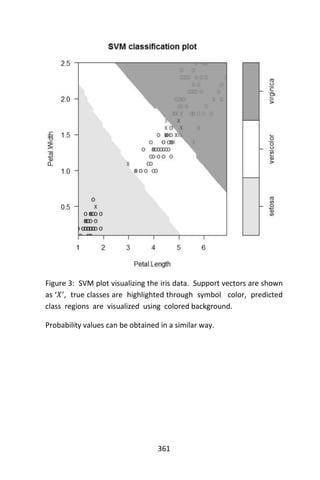

![363
17. Gradient boosting
Gradient boosting is a machine learning technique for regression
problems, which produces a prediction model in the form of an
ensemble of weak prediction models, typically decision trees. It builds
the model in a stage-wise fashion like other boosting methods do, and it
generalizes them by allowing optimization of an arbitrary differentiable
loss function. The gradient boosting method can also be used for
classification problems by reducing them to regression with a suitable
loss function.
The method was invented by Jerome H. Friedman in 1999 and was
published in a series of two papers, the first of which (Friedman, Greedy
Function Approximation: A Gradient Boosting Machine, 1995)
introduced the method, and the second one (Friedman, Stochastic
Gradient Boosting, 1999) described an important tweak to the
algorithm, which improves its accuracy and performance.
Algorithm
In many supervised learning problems one has an output variable y and
a vector of input variables 𝑥 connected together via a joint probability
distribution 𝑃(𝑥, 𝑦). Using a training set of known values of 𝑥 and
corresponding values of 𝑦, the goal is to find an approximation 𝐹̂(𝑥) to
a function 𝐹∗
(𝑥) that minimizes the expected value of some specified
loss function 𝐿(𝑦, 𝐹(𝑥)):
𝐹∗
= arg min
𝐹
𝔼 𝑥,𝑦[𝐿(𝑦, 𝐹(𝑥))]
Gradient boosting method assumes a real-valued 𝑦 and seeks an
approximation 𝐹̂(𝑥) in the form of a weighted sum of functions ℎᵢ(𝑥)
from some class ℋ, called base (or weak) learners:
𝐹(𝑥) = ∑ 𝛾𝑖ℎ𝑖(𝑥) + constant
𝑀
𝑖=1
.](https://image.slidesharecdn.com/048d9789-800e-4318-80f7-c96b1a8df646-150122193330-conversion-gate01/85/Predictive-Analytics-using-R-394-320.jpg)
![365
In pseudocode, the generic gradient boosting method is (Friedman,
Greedy Function Approximation: A Gradient Boosting Machine, 1995)
(Hastie, Tibshirani, & Friedman, 2009):
Input: training set {(𝑥𝑖, 𝑦𝑖)}𝑖=1
𝑛
, a differentiable loss function 𝐿(𝑦, 𝐹(𝑥))
number of iterations 𝑀.
Algorithm:
1. Initialize model with a constant value:
𝐹0(𝑥) = arg min
𝛾
∑ 𝐿(𝑦𝑖, 𝛾)
𝑛
𝑖=1
,
2. For 𝑚 = 1 to 𝑀:
a. Compute so-called pseudo-residuals:
𝑟𝑖𝑚 = − [
𝜕𝐿(𝑦𝑖, 𝐹(𝑥𝑖))
𝜕𝐹(𝑥𝑖)
]
𝐹(𝑥)=𝐹 𝑚−1(𝑥)
, 𝑓𝑜𝑟 𝑖 = 1, … 𝑛.
b. Fit a base learner ℎ 𝑚(𝑥) to pseudo-residuals, i.e. train it using
the training set {(𝑥𝑖, 𝑟𝑖𝑚)}𝑖=1
𝑛
.
c. Compute multiplier 𝛾 𝑚 by solving the following one-
dimensional optimization problem:
𝛾 𝑚 = arg min
𝛾
∑ 𝐿(𝑦𝑖, 𝐹 𝑚−1(𝑥𝑖) + 𝛾ℎ 𝑚(𝑥𝑖))
𝑛
𝑖=1
.
d. Update the model:
𝐹𝑚(𝑥) = 𝐹 𝑚−1(𝑥) + 𝛾 𝑚ℎ 𝑚(𝑥).
3. Output 𝐹𝑚(𝑥).](https://image.slidesharecdn.com/048d9789-800e-4318-80f7-c96b1a8df646-150122193330-conversion-gate01/85/Predictive-Analytics-using-R-396-320.jpg)


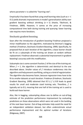
![371
on a linear model with backward-elimination for variable selection. The
resulting final model utilized hip circumference (hipcirc), knee breadth
(kneebreadth) and a compound covariate (anthro3a), which is defined
as the sum of the logarithmic measurements of chin skinfold, triceps
skinfold and subscapular skinfold:
> ## Reproduce formula of Garcia et al., 2005
> lm1 <- lm(DEXfat ~ hipcirc + kneebreadth + anthro3a, data
+ = bodyfat)
> coef(lm1)
(Intercept) hipcirc kneebreadth anthro3a
-75.2347840 0.5115264 1.9019904 8.9096375
A very similar model can be easily fitted by boosting, applying
glmboost() with default settings:
> ## Estimate same model by glmboost
> glm1 <- glmboost(DEXfat ~ hipcirc + kneebreadth +
+ anthro3a, data = bodyfat)
> coef(glm1, off2int=TRUE) ## off2int adds the offset to the
intercept
(Intercept) hipcirc kneebreadth anthro3a
-75.2073365 0.5114861 1.9005386 8.9071301
Note that in this case we used the default settings in control and the
default family Gaussian() leading to boosting with the 𝐿2 loss.
We now want to consider all available variables as potential predictors.
One way is to simply specify “.” on the right side of the formula:
> glm2 <- glmboost(DEXfat ~ ., data = bodyfat)
As an alternative one can explicitly provide the whole formula by using
the paste() function. Therefore, one could essentially call:
> preds <- names(bodyfat[, names(bodyfat) != “DEXfat”])
##names of predictors
> fm <- as.formula(paste(“DEXfat ~”, paste(preds, collapse
+ = “+”)))
## build formula](https://image.slidesharecdn.com/048d9789-800e-4318-80f7-c96b1a8df646-150122193330-conversion-gate01/85/Predictive-Analytics-using-R-402-320.jpg)
![372
> fm
+ DEXfat ~ age+waistcirc + hipcirc + elbowbreadth
+
+ kneebreadth + anthro3a + anthro3b + anthro3c +
+ anthro4
and provide fm to the formula argument in glmboost(). Note that a
solution using the paste() function is somewhat unavoidable when we
intend to combine different base-learners for plenty of predictors in
gamboost(). Note that at this iteration (mstop is still 100 as it is the
default value) anthro4a is not included in the resulting model as the
corresponding base-learner was never selected in the update step. The
function coef() by default only displays the selected variables but can
be forced to show all effects by specifying which = ““:
> coef(glm2, ## usually the argument ‘which’ is used to
## specify single base-
+ which = ““) ## learners via partial matching; With which
## = ““ we select all.
(Intercept) age waistcirc hipcirc elbowbreadth kneebreadth
-98.816608 0.0136 0.1897 0.3516 -0.384 1.7366
anthro3a anthro3b anthro3c anthro4
3.326860 3.6565 0.5954 0
attr(,”offset”)
[1] 30.78282
A plot of the coefficient paths, similar to the ones commonly known from
the LARS algorithm (Efron et al. 2004), can be easily produced by using
plot() on the glmboost object (see Figure 1):
> plot(glm2, off2int = TRUE) ## default plot, offset added
> ## to intercept
> ## now change ylim to the range of the coefficients
> ## without intercept (zoom-in)
> plot(glm2, ylim = range(coef(glm2, which = preds)))](https://image.slidesharecdn.com/048d9789-800e-4318-80f7-c96b1a8df646-150122193330-conversion-gate01/85/Predictive-Analytics-using-R-403-320.jpg)


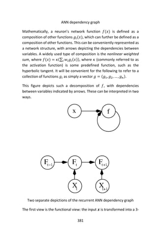

![383
The two views are largely equivalent. In either case, for this particular
network architecture, the components of individual layers are
independent of each other (e.g., the components of 𝑔 are independent
of each other given their input ℎ). This naturally enables a degree of
parallelism in the implementation.
Networks such as the previous one are commonly called feedforward,
because their graph is a directed acyclic graph. Networks with cycles are
commonly called recurrent. Such networks are commonly depicted in
the manner shown at the top of the figure, where 𝑓 is shown as being
dependent upon itself. However, an implied temporal dependence is not
shown.
Learning
What has attracted the most interest in neural networks is the possibility
of learning. Given a specific task to solve, and a class of functions 𝐹,
learning means using a set of observations to find 𝑓∗
∈ 𝐹 which solves
the task in some optimal sense.
This entails defining a cost function 𝐶: 𝐹 → ℝ such that, for the optimal
solution 𝑓∗
, 𝐶(𝑓∗) ≤ 𝐶(𝑓) ∀𝑓 ∈ 𝐹– i.e., no solution has a cost less than
the cost of the optimal solution.
The cost function 𝐶 is an important concept in learning, as it is a measure
of how far away a particular solution is from an optimal solution to the
problem to be solved. Learning algorithms search through the solution
space to find a function that has the smallest possible cost.
For applications where the solution is dependent on some data, the cost
must necessarily be a function of the observations, otherwise we would
not be modeling anything related to the data. It is frequently defined as
a statistic to which only approximations can be made. As a simple
example, consider the problem of finding the model 𝑓, which minimizes
𝐶 = 𝐸[(𝑓(𝑥) − 𝑦)2
], for data pairs (𝑥, 𝑦) drawn from some distribution
𝒟. In practical situations we would only have 𝑁 samples from 𝒟 and
thus, for the above example, we would only minimize 𝐶̂ =](https://image.slidesharecdn.com/048d9789-800e-4318-80f7-c96b1a8df646-150122193330-conversion-gate01/85/Predictive-Analytics-using-R-414-320.jpg)

![385
target value 𝑦 over all the example pairs. When one tries to minimize
this cost using gradient descent for the class of neural networks called
multilayer perceptrons, one obtains the common and well-known
backpropagation algorithm for training neural networks.
Tasks that fall within the paradigm of supervised learning are pattern
recognition (also known as classification) and regression (also known as
function approximation). The supervised learning paradigm is also
applicable to sequential data (e.g., for speech and gesture recognition).
This can be thought of as learning with a “teacher,” in the form of a
function that provides continuous feedback on the quality of solutions
obtained thus far.
Unsupervised learning
In unsupervised learning, some data 𝑥 is given and the cost function to
be minimized, that can be any function of the data 𝑥 and the network’s
output, 𝑓.
The cost function is dependent on the task (what we are trying to model)
and our a priori assumptions (the implicit properties of our model, its
parameters and the observed variables).
As a trivial example, consider the model 𝑓(𝑥) = 𝑎 where 𝑎 is a constant
and the cost 𝐶 = 𝐸[(𝑓(𝑥) − 𝑦)2
]. Minimizing this cost will give us a
value of 𝑎 that is equal to the mean of the data. The cost function can
be much more complicated. Its form depends on the application: for
example, in compression it could be related to the mutual information
between 𝑥 and 𝑓(𝑥), whereas in statistical modeling, it could be related
to the posterior probability of the model given the data. (Note that in
both of those examples those quantities would be maximized rather
than minimized).
Tasks that fall within the paradigm of unsupervised learning are in
general estimation problems; the applications include clustering, the
estimation of statistical distributions, compression and filtering.](https://image.slidesharecdn.com/048d9789-800e-4318-80f7-c96b1a8df646-150122193330-conversion-gate01/85/Predictive-Analytics-using-R-416-320.jpg)


![398
electromagnetic impulses between the neurons are studied.
Commonly used biological network simulators include Neuron, GENESIS,
NEST and Brian. Other simulators are XNBC and the NN Toolbox for
MATLAB.
Data analysis simulators
Unlike the research simulators, the data analysis simulators are intended
for practical applications of artificial neural networks. Their primary
focus is on data mining and forecasting. Data analysis simulators usually
have some form of preprocessing capabilities. Unlike the more general
development environments data analysis simulators use a relatively
simple static neural network that can be configured. A majority of the
data analysis simulators on the market use back propagating networks
or self-organizing maps as their core. The advantage of this type of
software is that it is relatively easy to use. Some data analysis simulators
are dedicated neural network packages, such as Neural Designer. Some
others work in conjunction with other computational environments,
such as NeuralTools for Microsoft Excel.
Simulators for teaching neural network theory
When the Parallel Distributed Processing volumes[1] [2][3] were
released in 1986-87, they provided some relatively simple software. The
original PDP software did not require any programming skills, which led
to its adoption by a wide variety of researchers in diverse fields. The
original PDP software was developed into a more powerful package
called PDP++, which in turn has become an even more powerful platform
called Emergent. With each development, the software has become
more powerful, but also more daunting for use by beginners.
In 1997, the tLearn software was released to accompany a book.[4] This
was a return to the idea of providing a small, user-friendly, simulator
that was designed with the novice in mind. tLearn allowed basic feed
forward networks, along with simple recurrent networks, both of which
can be trained by the simple back propagation algorithm. tLearn has not
been updated since 1999.](https://image.slidesharecdn.com/048d9789-800e-4318-80f7-c96b1a8df646-150122193330-conversion-gate01/85/Predictive-Analytics-using-R-429-320.jpg)


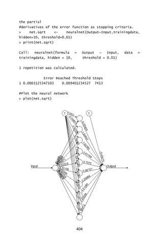
![405
#Test the neural network on some training data
> testdata <- as.data.frame((1:10)^2)
#Generate some squared numbers through the neural #network
#Lets see what properties net.sqrt has
> ls(net.results)
[1] “act.fct” “call” “covariate”
[4] “data” “err.fct” “generalized.weights”
[7] “linear.output” “model.list” “net.result”
[10] “response“ “result.matrix” “startweights”
[13] “weights”
#Lets see the results
> print(net.results$net.result)
[[1]]
[,1]
1 5.0490045485
2 7.4625475299
3 5.4268560491
4 9.3944183247
5 7.3261826045
6 9.7116754748
7 7.7005230133
8 6.1877876553
9 9.0208308800
10 5.7323789090
11 8.8662469974
12 9.6321471501
13 5.5556127899
14 8.8963448461
15 6.5228214924
16 4.6004103084
17 5.1903750160
18 7.4088926123
19 4.6820958475
20 8.7562521802
21 8.9002614981
22 9.9683150949
23 0.8709360456](https://image.slidesharecdn.com/048d9789-800e-4318-80f7-c96b1a8df646-150122193330-conversion-gate01/85/Predictive-Analytics-using-R-436-320.jpg)
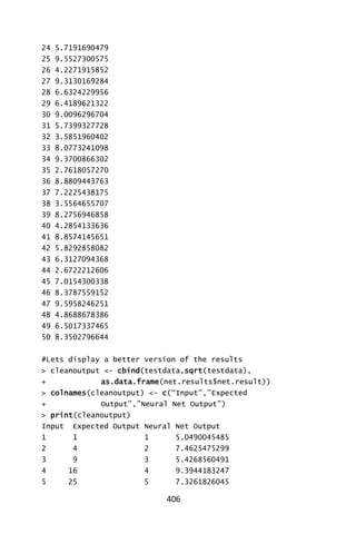
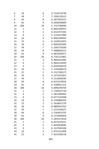


![423
(Rzepakowski & Jaroszewicz, 2010) produce the following uplift curves
using for the splice dataset (The SPLICE dataset: Classification, 2010).
Note: The R package entropy provides the functionality for performing
Kullback-Leibler (KL.plugin) and chi-squared (chi2.plugin) measures.
Given two samples from splice, we have:
> data1<-mydata[sample(1:nrow(mydata),100,replace=FALSE),]
> data2<-mydata[sample(1:nrow(mydata),100,replace=FALSE),]
> colnames(data1)[colnames(data1)==“RESP”] <- “RESP1”
> colnames(data2)[colnames(data2)==“RESP”] <- “RESP2”
> RESP1 = c(0.21, 0.24, 0.55)
> RESP2 = c(0.26, 0.25, 0.49)
> KL.plugin(RESP1, RESP2)
[1] 0.008884248 # the KL-distance
> chi2.plugin(RESP1,RESP2)
[1] 0.01736232 # the Chi2-distance](https://image.slidesharecdn.com/048d9789-800e-4318-80f7-c96b1a8df646-150122193330-conversion-gate01/85/Predictive-Analytics-using-R-454-320.jpg)


![426
depth, constrained on the arguments specified in
minsplit and minbucket.
bag.fraction the fraction of the training set observations randomly
selected for the purpose of fitting each tree in the forest.
minsplit the minimum number of observations that must exist in a
node in order for a split to be attempted.
minbucket_ct0 the minimum number of control observations in any
terminal <leaf> node.
minbucket_ct1 the minimum number of treatment observations in any
terminal <leaf> node.
keep.inbag if set to TRUE, an nrow(x) by ntree matrix is returned,
whose entries are the “in-bag” samples in each tree.
verbose print status messages?
Output
uplift: status messages enabled; set “verbose” to false to
disable
upliftRF: starting. Sat Jul 12 16:11:35 2014
10 out of 50 trees so far...
20 out of 50 trees so far...
30 out of 50 trees so far...
40 out of 50 trees so far...
predict
predict is a generic function for predictions from the results of various
model fitting functions. In this instance we use fit1 derived from fitting
the data with the upliftRF model.
> ### Fitted values on train data
> pred <- predict(fit1, dd)
> ### Compute uplift predictions
> uplift_pred <- pred[, 1] - pred[, 2]
> ### Put together data, predictions and add some dummy
> ### factors for illustration only
> dd2 <- data.frame(dd, uplift_pred, F1 = gl(2, 50, labels
+ = c(“A”, “B”)),
+ F2 = gl(4, 25, labels = c(“a”, “b”, “c”, “d”)))](https://image.slidesharecdn.com/048d9789-800e-4318-80f7-c96b1a8df646-150122193330-conversion-gate01/85/Predictive-Analytics-using-R-457-320.jpg)

![429
var rel.imp
1 X1 28.436811
2 X3 25.067272
3 X2 24.001705
4 X4 21.240306
5 X5 1.253906
Performance
This function provides a method for assessing performance for uplift
models (CRAN-project, 2012).
> dd_new <- sim_pte(n = 1000, p = 20, rho = 0, sigma =
+ sqrt(2), beta.den = 4)
> dd_new$treat <- ifelse(dd_new$treat == 1, 1, 0)
>
> pred <- predict(fit1, dd_new)
> perf <- performance(pred[, 1], pred[, 2], dd_new$y,
+ dd_new$treat, direction = 1)
> plot(perf[, 8] ~ perf[, 1], type =“l”, xlab = “Decile”,
+ ylab = “uplift”)](https://image.slidesharecdn.com/048d9789-800e-4318-80f7-c96b1a8df646-150122193330-conversion-gate01/85/Predictive-Analytics-using-R-460-320.jpg)


![443
but it’s not. It has order and length, but no dimensions (no rows, no
columns). R calls these kinds of objects “vectors” so you have to be
careful. In R, “matrices” have dimensions but “vectors” do not.
> jj[1] # the first element
[1] 0.71
> jj[84] # the last element
[1] 11.61
> jj[1:4] # the first 4 elements
[1] 0.71 0.63 0.85 0.44
> jj[-(1:80)] # everything EXCEPT the first 80 elements
[1] 16.20 14.67 16.02 11.61
> length(jj) # the number of elements
[1] 84
> dim(jj) # but no dimensions ...
NULL
> nrow(jj) # ... no rows
NULL
> ncol(jj) # ... and no columns
NULL
#-- if you want it to be a column vector (in R, a matrix),
# an easy way to go is:
> jjm = as.matrix(jj)
> dim(jjm)
[1] 84 1
Now, we will make a monthly time series object that starts in June of the
year 2293.
> options(digits=2) # the default is 7, but it’s
# more than I want now
> ?options # to see your options (it’s the
# help file)
> ?rnorm # we’re using it on the next line
> (zardoz = ts(rnorm(48), start=c(2293,6), frequency=12))
Jan Feb Mar Apr May Jun
2293 0.7068
2294 -0.7945 -0.3213 -0.6600 -1.7642 -0.1160 1.0249](https://image.slidesharecdn.com/048d9789-800e-4318-80f7-c96b1a8df646-150122193330-conversion-gate01/85/Predictive-Analytics-using-R-474-320.jpg)

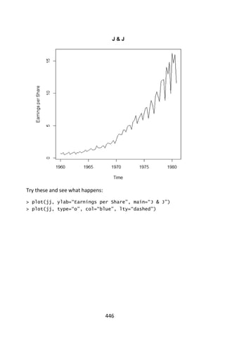
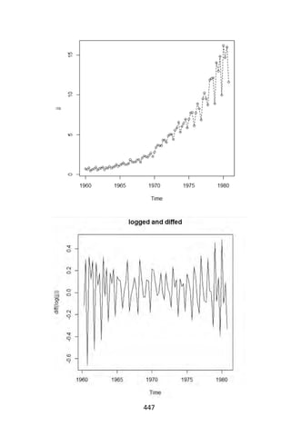

![449
# note- x and y are ts objects
#--- the help files [? and help() are the same]:
> ?plot.ts
> help(ts.plot)
> ?par # might as well skim the graphical
# parameters help file while you’re here
Note that if your data are a time series object, plot() will do the trick
(for a simple time plot, that is). Otherwise, plot.ts() will coerce the
graphic into a time plot.
We now look at filtering/smoothing the Johnson & Johnson series using
a two-sided moving average? Try this:
fjj(t)= ⅛ jj(t-2)+¼ jj(t-1)+¼ jj(t)+¼ jj(t+1)+⅛ jj(t+2)
and we’ll add a lowess (?lowess) fit for fun.
> k = c(.5,1,1,1,.5) # k is the vector of
# weights
> (k = k/sum(k))
[1] 0.12 0.25 0.25 0.25 0.12
> fjj = filter(jj, sides=2, k) # ?filter for help
> plot(jj)
> lines(fjj, col=“red”) # adds a line to the
# existing plot
> lines(lowess(jj), col=“blue”, lty=“dashed”)](https://image.slidesharecdn.com/048d9789-800e-4318-80f7-c96b1a8df646-150122193330-conversion-gate01/85/Predictive-Analytics-using-R-480-320.jpg)
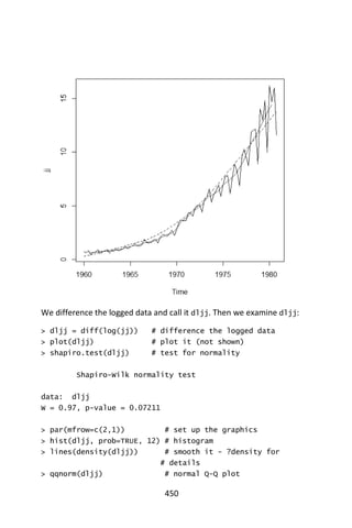
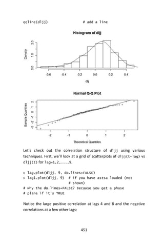
![452
Now let’s take a look at the ACF and PACF of dljj:
> par(mfrow=c(2,1)) # The power of accurate observation is
commonly called cynicism
# by those who have not got it. –
# George Bernard Shaw
> acf(dljj, 20) # ACF to lag 20 - no graph shown...
# keep reading
> pacf(dljj, 20) # PACF to lag 20 - no graph shown...
# keep reading
# !!NOTE!! acf2 on the line below is ONLY available in
# astsa and tsa3
> acf2(dljj) # this is what you’ll see below
ACF PACF
[1,] -0.51 -0.51
[2,] 0.07 -0.26](https://image.slidesharecdn.com/048d9789-800e-4318-80f7-c96b1a8df646-150122193330-conversion-gate01/85/Predictive-Analytics-using-R-483-320.jpg)
![453
[3,] -0.40 -0.70
[4,] 0.73 0.27
[5,] -0.37 0.16
[6,] 0.00 -0.11
[7,] -0.25 -0.01
[8,] 0.56 0.11
[9,] -0.28 0.05
[10,] -0.01 0.12
[11,] -0.22 -0.03
[12,] 0.45 -0.03
[13,] -0.21 0.04
[14,] -0.04 -0.08
[15,] -0.15 -0.04
[16,] 0.35 -0.04
[17,] -0.14 -0.04
[18,] -0.08 -0.06
[19,] -0.09 -0.02
[20,] 0.27 0.01](https://image.slidesharecdn.com/048d9789-800e-4318-80f7-c96b1a8df646-150122193330-conversion-gate01/85/Predictive-Analytics-using-R-484-320.jpg)

![455
Now we inspect the residuals. The third column of the resulting series
(the seasonal and trend components are in columns 1 and 2). Also, check
out the ACF of the residuals, acf(dog$time.series[,3]); the residuals
aren’t white—not even close. You can do a little (very little) better using
a local seasonal window, plot(dog <- stl(log(jj), s.win=4)), as
opposed to the global one used by specifying “per”. Type ?stl for
details. There is also something called StructTS that will fit parametric
structural models.
> dog$time.series[,3]
Qtr1 Qtr2 Qtr3 Qtr4
1960 0.02215 -0.08811 0.17311 -0.19320
1961 -0.02563 0.00128 0.15874 -0.11700
1962 -0.00070 0.00594 0.07749 -0.10622
1963 0.06021 -0.05831 0.03865 -0.00231](https://image.slidesharecdn.com/048d9789-800e-4318-80f7-c96b1a8df646-150122193330-conversion-gate01/85/Predictive-Analytics-using-R-486-320.jpg)
![456
1964 -0.01744 -0.03189 0.03428 0.02085
1965 -0.02364 0.00713 -0.01013 0.08639
1966 -0.07779 -0.07984 0.06758 0.11055
1967 -0.05578 -0.06423 -0.04485 0.19954
1968 -0.19148 0.02416 -0.02055 0.14136
1969 -0.07448 -0.00568 -0.01975 -0.01118
1970 -0.02523 0.04521 -0.05630 0.12087
1971 -0.07094 0.04718 -0.08955 0.04868
1972 0.04208 0.02030 -0.08487 0.00411
1973 0.03857 -0.00395 -0.00329 0.02490
1974 -0.00825 -0.00284 -0.03440 0.01659
1975 -0.00061 0.05262 -0.03305 -0.04415
1976 0.01273 0.09466 -0.08980 -0.06100
1977 0.07734 0.06977 -0.13041 -0.00992
1978 0.09135 0.04030 -0.04335 -0.12358
1979 0.14248 -0.01616 0.02089 -0.14976
1980 0.15572 0.00999 0.01320 -0.03985
> acf(dog$time.series[,3])
> (dog <- stl(log(jj), s.win=4))
Call:
stl(x = log(jj), s.window = 4)
Components
seasonal trend remainder
1960 Q1 0.01916 -0.4519 0.09023
1960 Q2 0.01526 -0.4462 -0.03109
1960 Q3 0.26000 -0.4405 0.01801](https://image.slidesharecdn.com/048d9789-800e-4318-80f7-c96b1a8df646-150122193330-conversion-gate01/85/Predictive-Analytics-using-R-487-320.jpg)


![462
Double integral: ∬(. )
closed interval: [𝑎, 𝑏]
open interval: (𝑎, 𝑏)
maximize: 𝑚𝑎𝑥(𝑎, 𝑏)
maximize subject to:
𝑚𝑖𝑛 𝑥
| 𝑐𝑜𝑛𝑑𝑖𝑡𝑖𝑜𝑛
minimize: 𝑚𝑖𝑛(𝑎, 𝑏)
Argument of the minimum:
arg min
𝑎∈𝐴
(. ) (.)
Laplace transform: ℒ
Weierstrass elliptic function: ℘
Natural logarithm: 𝑙𝑛(. )
Function: 𝑓(𝑥)
Composite function: 𝑓(𝑔(𝑥)),
𝑓 ∘ 𝑔
Iteration 𝑖 of 𝐹(𝑥): 𝐹𝑖(𝑥)
Combination: (
𝑛
𝑘
)
Factoiral: !
Distance between x and y:
||𝑥 − 𝑦||
If and only if: Iff, ↔, ⇔
approximately equal: ≈
Proportional to: ∝
Plur or minus: ±
Such that: :
Summation: ∑(. )
Double summation: ∑ ∑(. )
Sum from i=1,…,n: ∑ (. )𝑛
𝑖=1
Sum of all 𝑖 ∈ 𝑓(𝑖): ∑ (. )𝑖∈𝑓(𝑖)
Gradient: ∇
Not sign: ¬](https://image.slidesharecdn.com/048d9789-800e-4318-80f7-c96b1a8df646-150122193330-conversion-gate01/85/Predictive-Analytics-using-R-493-320.jpg)


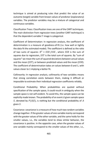


The document is a comprehensive book on predictive analytics authored by Dr. Jeffrey Strickland, highlighting his expertise in predictive modeling and statistical methods, alongside machine learning techniques. It serves as an advanced guide intended for readers with a fundamental understanding of mathematical statistics, detailing various predictive modeling methods and culminating in practical examples using R. The book is organized to first present statistical models, followed by machine learning approaches and specific applications such as uplift modeling and time series analysis.