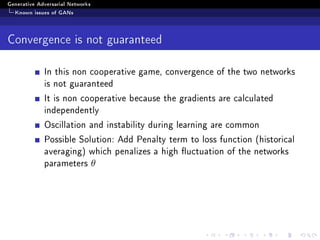
Generative Adversarial Networks (GANs) are a type of neural network that can generate new data with the same statistics as the training set. GANs work by having two neural networks - a generator and a discriminator - compete against each other in a minimax game framework. The generator tries to generate fake data that looks real, while the discriminator tries to tell apart the real data from the fake data. Wasserstein GANs introduce a new loss function based on the Wasserstein distance to help improve GAN training stability and convergence.

1. Generative Adversarial Networks
Generative Adversarial Networks
Benno Geiÿelmann
12. August 2018

2. Generative Adversarial Networks
Contents
1 General Architecture of GANs
2 The minimax problem
3 Approximating a solution for GANs
4 Known issues of GANs
5 Wasserstein GANs

3. Generative Adversarial Networks
General Architecture of GANs
Example
What does this look like?

4. Generative Adversarial Networks
General Architecture of GANs
Example

5. Generative Adversarial Networks
General Architecture of GANs
General Architecture of GANs

6. Generative Adversarial Networks
The minimax problem
The minimax problem
To retrieve a suitable generator network and a suitable discriminator
network, the following minimax problem needs to be solved:
min
G
max
D
V (D, G) = Ex∼pr(x)[log D(x)]+Ez∼pz(z)[log (1 − D(G(z)))]
with
D(x) = The discrimiator network
G(x) = The generator network
pr(x) = The distribution of the real data
pg(x) = The distribution of the generated data
pz(z) = The distribution of a random noise variable
Ex∼P [f(x)] = x P(x)f(x)

7. Generative Adversarial Networks
Approximating a solution for GANs
Approximating a solution for GANs
Algorithm 1: Gradient Descent for GAN
for it in interations do
nd ← {z(1), · · · , z(m)} ∼ pz(z)
rd ← {x(1), · · · , x(m)} ∼ pr(x)
gwd
← wd
1
m
m
i=1[log D(rd(i)) + log (1 − D(G(nd(i))))]
wd ← wd + ηgwd
nd ← {z(1), · · · , z(m)} ∼ pz(z)
gwg ← wg
1
m
m
i=1[log (1 − D(G(nd(i))))]
wg ← wg − ηgwg
end

8. Generative Adversarial Networks
Known issues of GANs
Convergence is not guaranteed
In this non cooperative game, convergence of the two networks
is not guaranteed
It is non cooperative because the gradients are calculated
independently
Oscillation and instability during learning are common
Possible Solution: Add Penalty term to loss function (historical
averaging) which penalizes a high uctuation of the networks
parameters θ

9. Generative Adversarial Networks
Known issues of GANs
Low dimensionality problem
In reality pr(x) is concentrating on a small subset of a possible
high dimensional event space
At the same time pg(x) is initialized using some low
dimensional noise data and is therefore also small
There can always be found a suitable discriminator D(x)

10. Generative Adversarial Networks
Known issues of GANs
Vanishing gradient problem
If we have a very good discriminator D(x) this means
D(G(z)) = 0 ∀z ∼ pz(z)
At the same time D(x) = 1 ∀x ∼ pr(r)
As we then have no gradient which we can minimize for the
generator, we cannot learn
Possible solution: Add Noise to input of discriminator to
articially enlarge its knowndistribution

11. Generative Adversarial Networks
Known issues of GANs
Mode collapse
It can happen that the generator outputs always the same
sample from pg(z)
We then end up in a small subset of the desired dirstibution
pr(x)
Variety of the created samples is very low
Possible solution: Show the discriminator a batch of outputs
from the generator (Minibatch discrimination)

12. Generative Adversarial Networks
Wasserstein GANs
Wasserstein GANs
Wasserstein GANs introduce a new way for measuring the
distance (and therefore also a new loss function) between two
distributions
In words the Wasserstein-1 Metric denes how costly it is to
transform a distribution Pr(x) into another distribution Pg(y)
using an optimal transport plan
Assuming that γ is this optimal transport plan where γ(x, y) is
the amount to transport from x to y, we can dene the total
cost as:
Cost =
x,y
γ(x, y)|x − y|

13. Generative Adversarial Networks
Wasserstein GANs
Wasserstein GANs
So the Wasserstein-1 metric is dened as:
W(Pr, Pg) = inf
γ∈Π(Pr,Pg)
E(x,y)∼γ[ x − y ]
Also called the earth moovers distance
Π(Pr, Pg) can be seen as the set of all possible transport plans
from Pr to Pg
Wasserstein metric needs the optimal transport plan (greatest
lower bound of these transport plans - the inmum)

14. Generative Adversarial Networks
Wasserstein GANs
Wasserstein GANs
The Wasserstein-1 is hard to be used within the GAN learning
process
Therefore there is used an equivalent denition derived from
Kantorovich-Rubinstein duality
W(Pr, Pg) = sup
f L≤1
Ex∼Pr [f(x)] − Ex∼Pg [f(x)]
where f must be a 1-Lipschitz function.
f(x) can be seen as an instance of a parameterized family of
functions {fw(x)}w∈W

15. Generative Adversarial Networks
Wasserstein GANs
Wasserstein GANs
The discriminator now has the task to learn this function again
as a neural network
Actually the discriminator (or now called critic) has the aim to
learn the Wasserstein-1 distance:
W(Pr, Pg) = max
w∈W
Ex∼Pr [fw(x)] − Ez∼Pz [fw(G(z))]
At the same time for a xed f at time t the generator wants
to miniminize W(Pr, Pg) and does this by descending on
W(Pr, Pg)

16. Generative Adversarial Networks
Wasserstein GANs
Wasserstein GANs