Administrivia
• HW4 willbe released in parts. All of it is due together in about 3 weeks.
• Part 1 on Decision trees and ensemble methods will be released
tomorrow.
• Project details will be released early next week.
• Groups of 4 (start forming groups).
• Today’s plan:
• Decision trees
• Ensemble methods
Decision trees
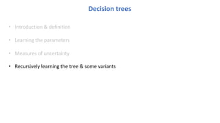
• Introduction& definition
• Learning the parameters
• Measures of uncertainty
• Recursively learning the tree & some variants
5.
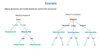
We have seendifferent ML models for classification/regression:
• linear models, nonlinear models induced by kernels, neural networks
Decision tree is another popular one:
• nonlinear in general
• works for both classification and regression; we focus on classification
• one key advantage is good interpretability
• ensembles of trees are very effective
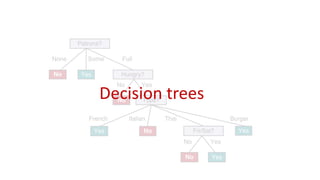
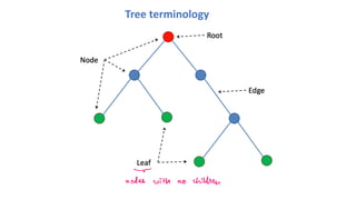
Decision trees
Tree terminology
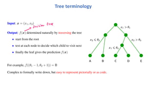
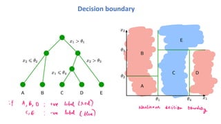
Input: x= (x1, x2)
Output: f(x) determined naturally by traversing the tree
• start from the root
• test at each node to decide which child to visit next
• finally the leaf gives the prediction f(x)
For example, f((θ1 − 1, θ2 + 1)) = B
Complex to formally write down, but easy to represent pictorially or as code.
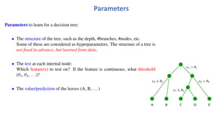
Parameters
Parameters to learnfor a decision tree:
• The structure of the tree, such as the depth, #branches, #nodes, etc.
Some of these are considered as hyperparameters. The structure of a tree is
not fixed in advance, but learned from data.
• The test at each internal node:
Which feature(s) to test on? If the feature is continuous, what threshold
(θ1, θ2, . . .)?
• The value/prediction of the leaves (A, B, . . .)
11.
Decision trees
• Introduction& definition
• Learning the parameters
• Measures of uncertainty
• Recursively learning the tree & some variants
12.
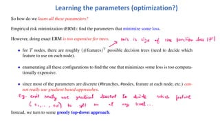
Learning the parameters(optimization?)
So how do we learn all these parameters?
Empirical risk minimization (ERM): find the parameters that minimize some loss.
However, doing exact ERM is too expensive for trees.
• for T nodes, there are roughly (#features)T
possible decision trees (need to decide which
feature to use on each node).
• enumerating all these configurations to find the one that minimizes some loss is too computa-
tionally expensive.
• since most of the parameters are discrete (#branches, #nodes, feature at each node, etc.) can-
not really use gradient based approaches.
Instead, we turn to some greedy top-down approach.
13.
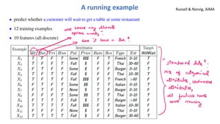
A running exampleRussell & Norvig, AIMA
• predict whether a customer will wait to get a table at some restaurant
• 12 training examples
• 10 features (all discrete)
14.
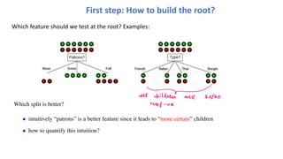
First step: Howto build the root?
Which feature should we test at the root? Examples:
Which split is better?
• intuitively “patrons” is a better feature since it leads to “more certain” children
• how to quantify this intuition?
15.
Decision trees
• Introduction& definition
• Learning the parameters
• Measures of uncertainty
• Recursively learning the tree & some variants
16.
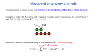
The uncertainity ofa node should be a function of the distribution of the classes within the node.
Example: a node with 2 positive and 4 negative examples can be summarized by a distribution P
with P(Y = +1) = 1/3 and P(Y = −1) = 2/3
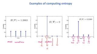
One classic measure of the uncertainity of a distribution is its (Shannon) entropy:
H(P) = −
C
!
k=1
P(Y = k) log P(Y = k)
Measure of uncertainty of a node
17.
H(P) = EY∼P
!
log
"
1
P(Y )
#$
=
C
%
k=1
P(Y = k) log
"
1
P(Y = k)
#
= −
C
%
k=1
P(Y = k) log P(Y = k)
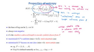
• the base of log can be 2, e or 10
• always non-negative
• it’s the smallest codeword length to encode symbols drawn from P
• maximized if P is uniform (max = ln C): most uncertain case
• minimized if P focuses on one class (min = 0): most certain case
• e.g. P = (1, 0, . . . , 0)
• 0 log 0 is defined naturally as limz→0+ z log z = 0
Properties of entropy
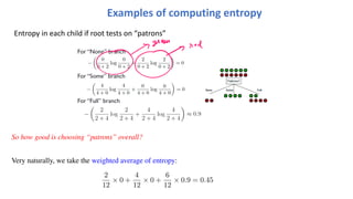
Examples of computingentropy
Entropy in each child if root tests on “patrons”
So how good is choosing “patrons” overall?
Very naturally, we take the weighted average of entropy:
2
12
× 0 +
4
12
× 0 +
6
12
× 0.9 = 0.45
20.
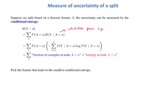
Suppose we splitbased on a discrete feature A, the uncertainty can be measured by the
conditional entropy:
H(Y | A)
=
!
a
P(A = a)H(Y | A = a)
=
!
a
P(A = a)
"
−
C
!
k=1
P(Y | A = a) log P(Y | A = a)
#
=
!
a
“fraction of examples at node A = a” × “entropy at node A = a”
Pick the feature that leads to the smallest conditional entropy.
Measure of uncertainty of a split
21.
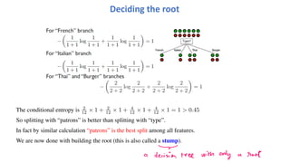
The conditional entropyis 2
12 × 1 + 2
12 × 1 + 4
12 × 1 + 4
12 × 1 = 1 > 0.45
So splitting with “patrons” is better than splitting with “type”.
In fact by similar calculation “patrons” is the best split among all features.
We are now done with building the root (this is also called a stump).
Deciding the root
22.
Decision trees
• Introduction& definition
• Learning the parameters
• Measures of uncertainty
• Recursively learning the tree & some variants
23.
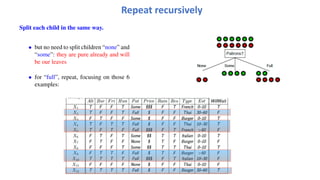
Split each childin the same way.
• but no need to split children “none” and
“some”: they are pure already and will
be our leaves
• for “full”, repeat, focusing on those 6
examples:
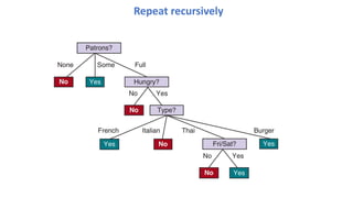
Repeat recursively
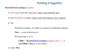
Putting it together
DecisionTreeLearning(Examples)
•if Examples have the same class, return a leaf with this class
• else if Examples is empty, return a leaf with majority class of parent
• else
find the best feature A to split (e.g. based on conditional entropy)
Tree ← a root with test on A
For each value a of A:
Child ← DecisionTreeLearning(Examples with A = a)
add Child to Tree as a new branch
• return Tree
26.
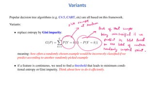
Popular decision treealgorithms (e.g. C4.5, CART, etc) are all based on this framework.
Variants:
• replace entropy by Gini impurity:
G(P) =
C
!
k=1
P(Y = k)(1 − P(Y = k))
meaning: how often a randomly chosen example would be incorrectly classified if we
predict according to another randomly picked example
• if a feature is continuous, we need to find a threshold that leads to minimum condi-
tional entropy or Gini impurity. Think about how to do it efficiently.
Variants
27.
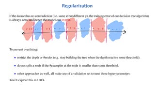
If the datasethas no contradiction (i.e. same x but different y), the training error of our decision tree algorithm
is always zero, and hence the model can overfit.
To prevent overfitting:
• restrict the depth or #nodes (e.g. stop building the tree when the depth reaches some threshold).
• do not split a node if the #examples at the node is smaller than some threshold.
• other approaches as well, all make use of a validation set to tune these hyperparameters
You’ll explore this in HW4.
Regularization
Acknowledgement
We borrow someof the content from Stanford’s CS229
slides on Ensemble Methods, by Nandita Bhaskhar:
https://cs229.stanford.edu/lectures-spring2022/cs229-
boosting_slides.pdf
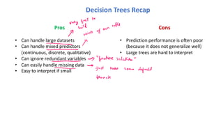
Pros
• Can handlelarge datasets
• Can handle mixed predictors
(continuous, discrete, qualitative)
• Can ignore redundant variables
• Can easily handle missing data
• Easy to interpret if small
Cons
• Prediction performance is often poor
(because it does not generalize well)
• Large trees are hard to interpret
Decision Trees Recap
32.
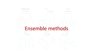
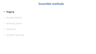
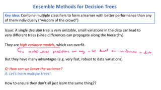
Ensemble Methods forDecision Trees
Issue: A single decision tree is very unstable, small variations in the data can lead to
very different trees (since differences can propagate along the hierarchy).
They are high variance models, which can overfit.
But they have many advantages (e.g. very fast, robust to data variations).
Q: How can we lower the variance?
A: Let’s learn multiple trees!
How to ensure they don’t all just learn the same thing??
Key idea: Combine multiple classifiers to form a learner with better performance than any
of them individually (“wisdom of the crowd”)
33.
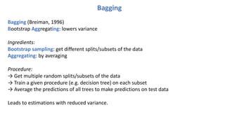
Bagging
Bagging (Breiman, 1996)
BootstrapAggregating: lowers variance
Ingredients:
Bootstrap sampling: get different splits/subsets of the data
Aggregating: by averaging
Procedure:
→ Get multiple random splits/subsets of the data
→ Train a given procedure (e.g. decision tree) on each subset
→ Average the predictions of all trees to make predictions on test data
Leads to estimations with reduced variance.
34.
Bagging
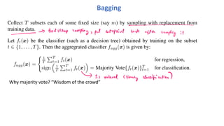
Collect T subsetseach of some fixed size (say m) by sampling with replacement from
training data.
Let ft(x) be the classifier (such as a decision tree) obtained by training on the subset
t ∈ {1, . . . , T}. Then the aggregrated classifier fagg(x) is given by:
fagg(x) =
! 1
T
"T
t=1 ft(x) for regression,
sign
#
1
T
"T
t=1 ft(x)
$
= Majority Vote{ft(x)}T
t=1 for classification.
Why majority vote? “Wisdom of the crowd”
35.
Bagging
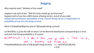
Why majority vote?“Wisdom of the crowd”
Suppose I ask each of you: “Will the stock market go up tomorrow?”
Suppose each of you has a 60% chance of being correct, and all of you make
independent predictions (probability of any 1 person being correct is independent of
probability of any one else being correct).
What is Probability(Majority vote of 100 people being correct)?
Let BinCDF(!, #, $) be the CDF at value ! of the Binomial distribution corresponding to # trials
and each trial having probability $ of success
Probability(Majority vote of 100 people being correct) = 1 – BinCDF(50,100,0.6)
≈ 0.97
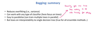
• Reduces overfitting(i.e., variance)
• Can work with any type of classifier (here focus on trees)
• Easy to parallelize (can train multiple trees in parallel)
• But loses on interpretability to single decision tree (true for all ensemble methods..)
Bagging: summary
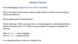
Issue with bagging:Bagged trees are still too correlated
Each is trained on large enough random sample of data and often end up not being
sufficiently different.
How to decorrelate the trees further?
Simple technique: When growing a tree on a bootstrapped (i.e. subsampled) dataset,
before each split select ! ≤ # of the # input variables at random as candidates for
splitting.
When ! = # → same as Bagging
When ! < # → Random forests
! is a hyperparameter, tuned via a validation set.
Random forests
40.
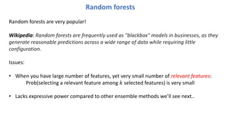
Random forests arevery popular!
Wikipedia: Random forests are frequently used as "blackbox" models in businesses, as they
generate reasonable predictions across a wide range of data while requiring little
configuration.
Issues:
• When you have large number of features, yet very small number of relevant features:
Prob(selecting a relevant feature among ! selected features) is very small
• Lacks expressive power compared to other ensemble methods we’ll see next..
Random forests
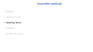
Boosting
Recall that thebagged/random forest classifier is given by
fagg(x) = sign
!
1
T
T
"
t=1
ft(x)
#
where each {ft}T
t=1 belongs to the function class F (such as a decision tree), and is trained
in parallel.
Instead of training the {ft}T
t=1 in parallel, what if we sequentially learn which models to
use from the function class F so that they are together as accurate as possible?
More formally, what is the best classifier sign (h(x)), where
h(x) =
T
"
t=1
βtft(x) for βt ≥ 0 and ft ∈ F.
Boosting is a way of doing this.
43.
Boosting
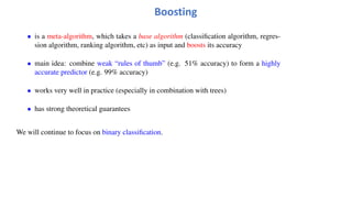
• is ameta-algorithm, which takes a base algorithm (classification algorithm, regres-
sion algorithm, ranking algorithm, etc) as input and boosts its accuracy
• main idea: combine weak “rules of thumb” (e.g. 51% accuracy) to form a highly
accurate predictor (e.g. 99% accuracy)
• works very well in practice (especially in combination with trees)
• has strong theoretical guarantees
We will continue to focus on binary classification.
44.
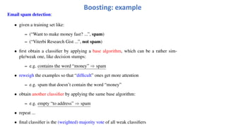
Email spam detection:
•given a training set like:
– (“Want to make money fast? ...”, spam)
– (“Viterbi Research Gist ...”, not spam)
• first obtain a classifier by applying a base algorithm, which can be a rather sim-
ple/weak one, like decision stumps:
– e.g. contains the word “money” ⇒ spam
• reweigh the examples so that “difficult” ones get more attention
– e.g. spam that doesn’t contain the word “money”
• obtain another classifier by applying the same base algorithm:
– e.g. empty “to address” ⇒ spam
• repeat ...
• final classifier is the (weighted) majority vote of all weak classifiers
Boosting: example
45.
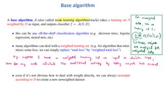
A base algorithmA (also called weak learning algorithm/oracle) takes a training set S
weighted by D as input, and outputs classifier f ← A(S, D)
• this can be any off-the-shelf classification algorithm (e.g. decision trees, logistic
regression, neural nets, etc)
• many algorithms can deal with a weighted training set (e.g. for algorithm that mini-
mizes some loss, we can simply replace “total loss” by “weighted total loss”)
• even if it’s not obvious how to deal with weight directly, we can always resample
according to D to create a new unweighted dataset
Base algorithm
46.
Boosting: Idea
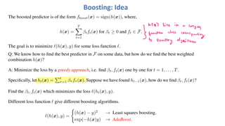
The boostedpredictor is of the form fboost(x) = sign(h(x)), where,
h(x) =
T
!
t=1
βtft(x) for βt ≥ 0 and ft ∈ F.
The goal is to minimize "(h(x), y) for some loss function ".
Q: We know how to find the best predictor in F on some data, but how do we find the best weighted
combination h(x)?
A: Minimize the loss by a greedy approach, i.e. find βt, ft(x) one by one for t = 1, . . . , T.
Specifically, let ht(x) =
"t
τ=1 βτ fτ (x). Suppose we have found ht−1(x), how do we find βt, ft(x)?
Find the βt, ft(x) which minimizes the loss "(ht(x), y).
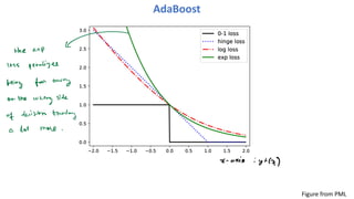
Different loss function " give different boosting algorithms.
"(h(x), y) =
#
(h(x) − y)2
→ Least squares boosting,
exp(−h(x)y) → AdaBoost.
AdaBoost
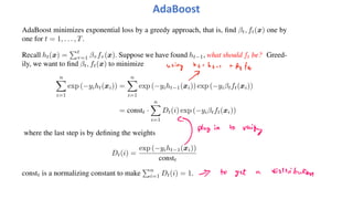
AdaBoost minimizes exponentialloss by a greedy approach, that is, find βt, ft(x) one by
one for t = 1, . . . , T.
Recall ht(x) =
!t
τ=1 βτ fτ (x). Suppose we have found ht−1, what should ft be? Greed-
ily, we want to find βt, ft(x) to minimize
n
"
i=1
exp (−yiht(xi)) =
n
"
i=1
exp (−yiht−1(xi)) exp (−yiβtft(xi))
= constt ·
n
"
i=1
Dt(i) exp (−yiβtft(xi))
where the last step is by defining the weights
Dt(i) =
exp (−yiht−1(xi))
constt
constt is a normalizing constant to make
!n
i=1 Dt(i) = 1.
50.
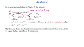
AdaBoost
So the goalbecomes finding βt, ft(x) ∈ F that minimize
n
!
i=1
Dt(i) exp (−yiβtft(xi))
=
!
i:yi!=ft(xi)
Dt(i)eβt
+
!
i:yi=ft(xi)
Dt(i)e−βt
= "teβt
+ (1 − "t)e−βt
(where "t =
"
n:yi!=ft(xi) Dt(i) is weighted error of ft)
= "t(eβt
− e−βt
) + e−βt
Therefore, we should find ft(x) to minimize its the weighted classification error "t (what
we expect the base algorithm to do intuitively).
51.
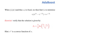
When ft(x) (andthus !t) is fixed, we then find βt to minimize
!t(eβt
− e−βt
) + e−βt
Exercise: verify that the solution is given by:
βt =
1
2
ln
!
1 − !t
!t
"
Hint: ex
is a convex function of x.
AdaBoost
52.
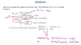
How do weupdate the weights for the next step? The definition of Dt+1(i) is actually
recursive,
Dt+1(i) =
exp (−yiht(xi))
constt+1
=
exp (−yiht−1(xi))
constt+1
· exp (−yiβtft(xi))
=
!
Dt(i)
constt
constt+1
"
· exp (−yiβtft(xi))
=⇒ Dt+1(i) ∝ Dt(i) exp(−βtyift(xi)) =
#
Dt(i)e−βt
if ft(xi) = yi
Dt(i)eβt
else
AdaBoost
53.
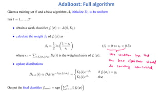
Given a trainingset S and a base algorithm A, initialize D1 to be uniform
For t = 1, . . . , T
• obtain a weak classifier ft(x) ← A(S, Dt)
• calculate the weight βt of ft(x) as
βt =
1
2
ln
!
1 − "t
"t
"
(βt > 0 ⇔ "t < 0.5)
where "t =
#
i:ft(xi)!=yi
Dt(i) is the weighted error of ft(x).
• update distributions
Dt+1(i) ∝ Dt(i)e−βtyift(xi)
=
$
Dt(i)e−βt
if ft(xi) = yi
Dt(i)eβt
else
Output the final classifier fboost = sgn
%#T
t=1 βtft(x)
&
AdaBoost: Full algorithm
54.
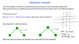
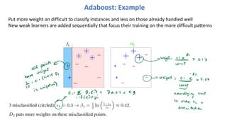
Put more weighton difficult to classify instances and less on those already handled well
New weak learners are added sequentially that focus their training on the more difficult patterns
Adaboost: Example
10 data points in R2
The size of + or - indicates the weight, which starts from uniform D1
Toy Example
Toy Example
Toy Example
Toy Example
Toy Example
D1
weak classifiers = vertical or h
Base algorithm is decision stump:
Observe that no stump can predict very accurately for this dataset.
55.
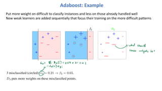
Put more weighton difficult to classify instances and less on those already handled well
New weak learners are added sequentially that focus their training on the more difficult patterns
Round 1
Round 1
Round 1
Round 1
Round 1
h1
!
"1
1
=0.30
=0.42
2
D
Adaboost: Example
3 misclassified (circled): !1 = 0.3 → β1 = 1
2 ln
!
1−!t
!t
"
≈ 0.42.
D2 puts more weights on these misclassified points.
(!
56.
Put more weighton difficult to classify instances and less on those already handled well
New weak learners are added sequentially that focus their training on the more difficult patterns
Round 2
Round 2
Round 2
Round 2
Round 2
!
"2
2
=0.21
=0.65
h2 3
D
Adaboost: Example
3 misclassified (circled): !2 = 0.21 → β2 = 0.65.
D3 puts more weights on these misclassified points.
("
57.
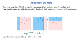
Put more weighton difficult to classify instances and less on those already handled well
New weak learners are added sequentially that focus their training on the more difficult patterns
Round 3
Round 3
Round 3
Round 3
Round 3
h3
!
"3
3=0.92
=0.14
Adaboost: Example
again 3 misclassified (circled): !3 = 0.14 → β3 = 0.92.
(#
58.
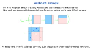
Put more weighton difficult to classify instances and less on those already handled well
New weak learners are added sequentially that focus their training on the more difficult patterns
All data points are now classified correctly, even though each weak classifier makes 3 mistakes.
Final Classifier
Final Classifier
Final Classifier
Final Classifier
Final Classifier
H
final
+ 0.92
+ 0.65
0.42
sign
=
=
Adaboost: Example


![[Women in Data Science Meetup ATX] Decision Trees](https://cdn.slidesharecdn.com/ss_thumbnails/decisiontrees-161118165341-thumbnail.jpg?width=640&height=640&fit=bounds)


![Hacking-Uncovered-How-People-Get-Hacked-and-How-to-Stay-Safe[1].pptx](https://cdn.slidesharecdn.com/ss_thumbnails/hacking-uncovered-how-people-get-hacked-and-how-to-stay-safe1-260130170011-4883a9c7-thumbnail.jpg?width=640&height=640&fit=bounds)


![7.__Developing_a_Research_Proposal[1].pptx](https://cdn.slidesharecdn.com/ss_thumbnails/7-260131073037-df92dd7d-thumbnail.jpg?width=640&height=640&fit=bounds)


