The document discusses the application of gradient boosted regression trees (GBRT) using the scikit-learn library, emphasizing its advantages and disadvantages in machine learning. It provides a detailed overview of gradient boosting techniques, how to implement them in scikit-learn, and includes a case study on California housing data to illustrate practical usage and challenges. Additionally, it covers hyperparameter tuning, model interpretation, and techniques for avoiding overfitting.

1. Gradient Boosted Regression Trees
scikit
Peter Prettenhofer (@pprett)
Gilles Louppe (@glouppe)
DataRobot
Universit´ de Li`ge, Belgium
e
e

2. Motivation

3. Motivation

4. Outline
1 Basics
2 Gradient Boosting
3 Gradient Boosting in Scikit-learn
4 Case Study: California housing

5. About us
Peter
• @pprett
• Python & ML ∼ 6 years
• sklearn dev since 2010
Gilles
• @glouppe
• PhD student (Li`ge,
e
Belgium)
• sklearn dev since 2011
Chief tree hugger

6. Outline
1 Basics
2 Gradient Boosting
3 Gradient Boosting in Scikit-learn
4 Case Study: California housing

7. Machine Learning 101
• Data comes as...
• A set of examples {(xi , yi )|0 ≤ i < n samples}, with
• Feature vector x ∈ Rn features , and
• Response y ∈ R (regression) or y ∈ {−1, 1} (classification)
• Goal is to...
• Find a function y = f (x)
ˆ
• Such that error L(y , y ) on new (unseen) x is minimal
ˆ

8. Classification and Regression Trees [Breiman et al, 1984]
MedInc <= 5.04
MedInc <= 3.07
AveRooms <= 4.31
1.62
1.16
MedInc <= 6.82
AveOccup <= 2.37
AveOccup <= 2.74
2.79
1.88
3.39
2.56
sklearn.tree.DecisionTreeClassifier|Regressor
MedInc <= 7.82
3.73
4.57

9. Function approximation with Regression Trees
10
8
6
ground truth
RT d=1
RT d=3
RT d=20
4
y
2
0
2
4
6
8
0
2
4
x
6
8
10

10. Function approximation with Regression Trees
10
8
6
ground truth
RT d=1
RT d=3
RT d=20
4
Deprecated
y
2
0
• Nowadays seldom used alone
2
• Ensembles: Random Forest, Bagging, or Boosting
(see sklearn.ensemble)
4
6
8
0
2
4
x
6
8
10

11. Outline
1 Basics
2 Gradient Boosting
3 Gradient Boosting in Scikit-learn
4 Case Study: California housing

12. Gradient Boosted Regression Trees
Advantages
• Heterogeneous data (features measured on different scale),
• Supports different loss functions (e.g. huber),
• Automatically detects (non-linear) feature interactions,
Disadvantages
• Requires careful tuning
• Slow to train (but fast to predict)
• Cannot extrapolate

13. Boosting
AdaBoost [Y. Freund & R. Schapire, 1995]
• Ensemble: each member is an expert on the errors of its
predecessor
• Iteratively re-weights training examples based on errors
2
x1
1
0
1
2
2
1
0
x0
1
2
3
2
1
0
x0
1
2
3
2
1
0
x0
1
2
sklearn.ensemble.AdaBoostClassifier|Regressor
3
2
1
0
x0
1
2
3

14. Boosting
Huge success
AdaBoost [Y. Freund & R. Schapire, 1995]
• Viola-Jones Face Detector (2001)
• Ensemble: each member is an expert on the errors of its
predecessor
• Iteratively re-weights training examples based on errors
2
x1
1
0
1
2
2
1
0
x0
1
2
3
2
1
0
x0
1
2
3
2
1
0
x0
1
2
3
2
1
• Freund & Schapire won the G¨del prize 2003
o
sklearn.ensemble.AdaBoostClassifier|Regressor
0
x0
1
2
3

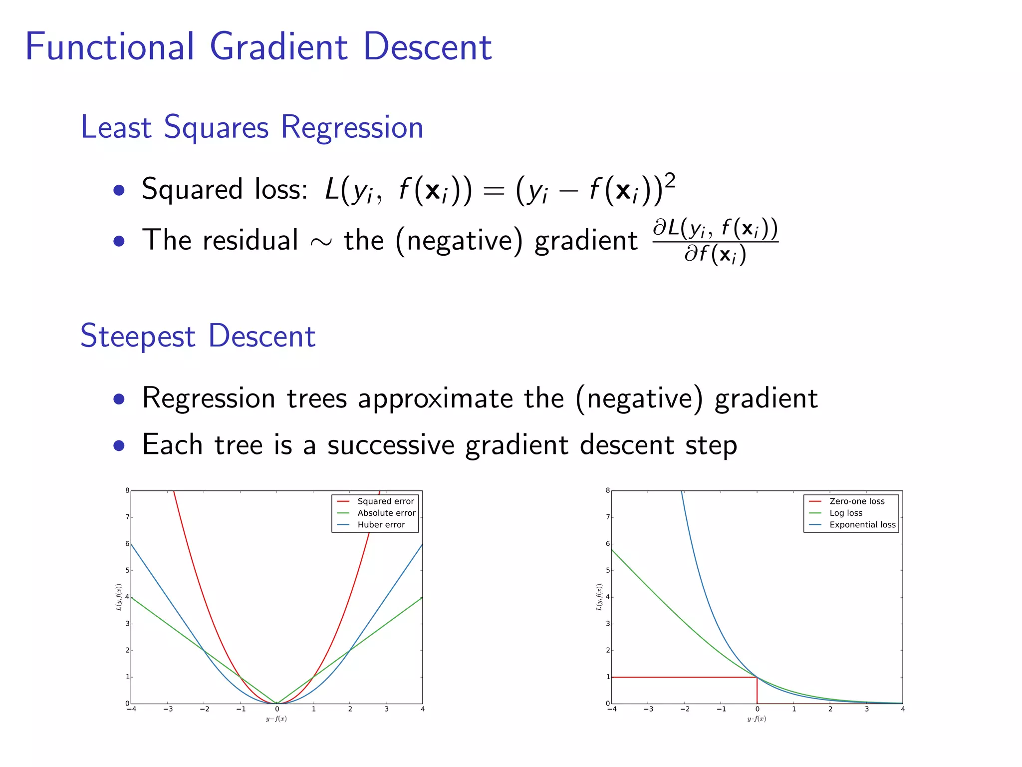
15. Gradient Boosting [J. Friedman, 1999]
Statistical view on boosting
• ⇒ Generalization of boosting to arbitrary loss functions

16. Gradient Boosting [J. Friedman, 1999]
Statistical view on boosting
• ⇒ Generalization of boosting to arbitrary loss functions
y
Residual fitting
2.5
2.0
1.5
1.0
0.5
0.0
0.5
1.0
1.5
2.0
Ground truth
tree 1
+
∼
2
x
6
10
tree 2
2
x
6
10
tree 3
+
2
x
6
10
2
sklearn.ensemble.GradientBoostingClassifier|Regressor
x
6
10

17. Functional Gradient Descent
Least Squares Regression
• Squared loss: L(yi , f (xi )) = (yi − f (xi ))2
f
• The residual ∼ the (negative) gradient ∂L(yi ,(x (xi ))
∂f i )

18. Functional Gradient Descent
Least Squares Regression
• Squared loss: L(yi , f (xi )) = (yi − f (xi ))2
f
• The residual ∼ the (negative) gradient ∂L(yi ,(x (xi ))
∂f i )
Steepest Descent
• Regression trees approximate the (negative) gradient
• Each tree is a successive gradient descent step
8
8
Squared error
Absolute error
Huber error
7
6
6
5
L(y,f(x))
5
L(y,f(x))
Zero-one loss
Log loss
Exponential loss
7
4
4
3
3
2
2
1
0
1
4
3
2
1
0
y−f(x)
1
2
3
4
0
4
3
2
1
0
y ·f(x)
1
2
3
4

19. Outline
1 Basics
2 Gradient Boosting
3 Gradient Boosting in Scikit-learn
4 Case Study: California housing

20. GBRT in scikit-learn
How to use it
>>> from sklearn.ensemble import GradientBoostingClassifier
>>> from sklearn.datasets import make_hastie_10_2
>>> X, y = make_hastie_10_2(n_samples=10000)
>>> est = GradientBoostingClassifier(n_estimators=200, max_depth=3)
>>> est.fit(X, y)
...
>>> # get predictions
>>> pred = est.predict(X)
>>> est.predict_proba(X)[0] # class probabilities
array([ 0.67, 0.33])
Implementation
• Written in pure Python/Numpy (easy to extend).
• Builds on top of sklearn.tree.DecisionTreeRegressor (Cython).
• Custom node splitter that uses pre-sorting (better for shallow trees).

21. Example
from sklearn.ensemble import GradientBoostingRegressor
est = GradientBoostingRegressor(n_estimators=2000, max_depth=1).fit(X, y)
for pred in est.staged_predict(X):
plt.plot(X[:, 0], pred, color=’r’, alpha=0.1)
10
8
6
ground truth
RT d=1
RT d=3
GBRT d=1
High bias - low variance
4
y
2
0
2
4
Low bias - high variance
6
8
0
2
4
x
6
8
10

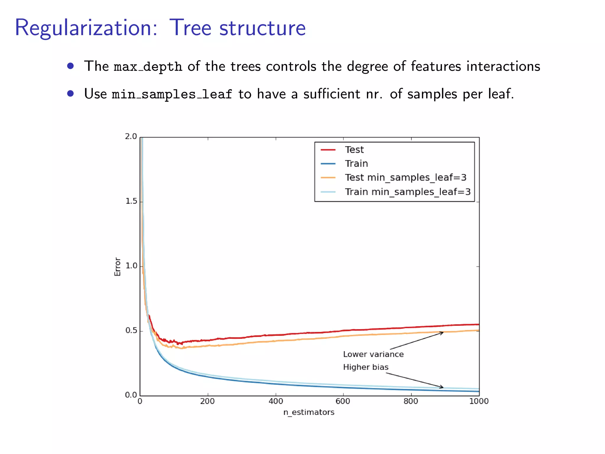
22. Model complexity & Overfitting
test_score = np.empty(len(est.estimators_))
for i, pred in enumerate(est.staged_predict(X_test)):
test_score[i] = est.loss_(y_test, pred)
plt.plot(np.arange(n_estimators) + 1, test_score, label=’Test’)
plt.plot(np.arange(n_estimators) + 1, est.train_score_, label=’Train’)
2.0
Test
Train
Error
1.5
1.0
Lowest test error
0.5
train-test gap
0.0
0
200
400
n_estimators
600
800
1000

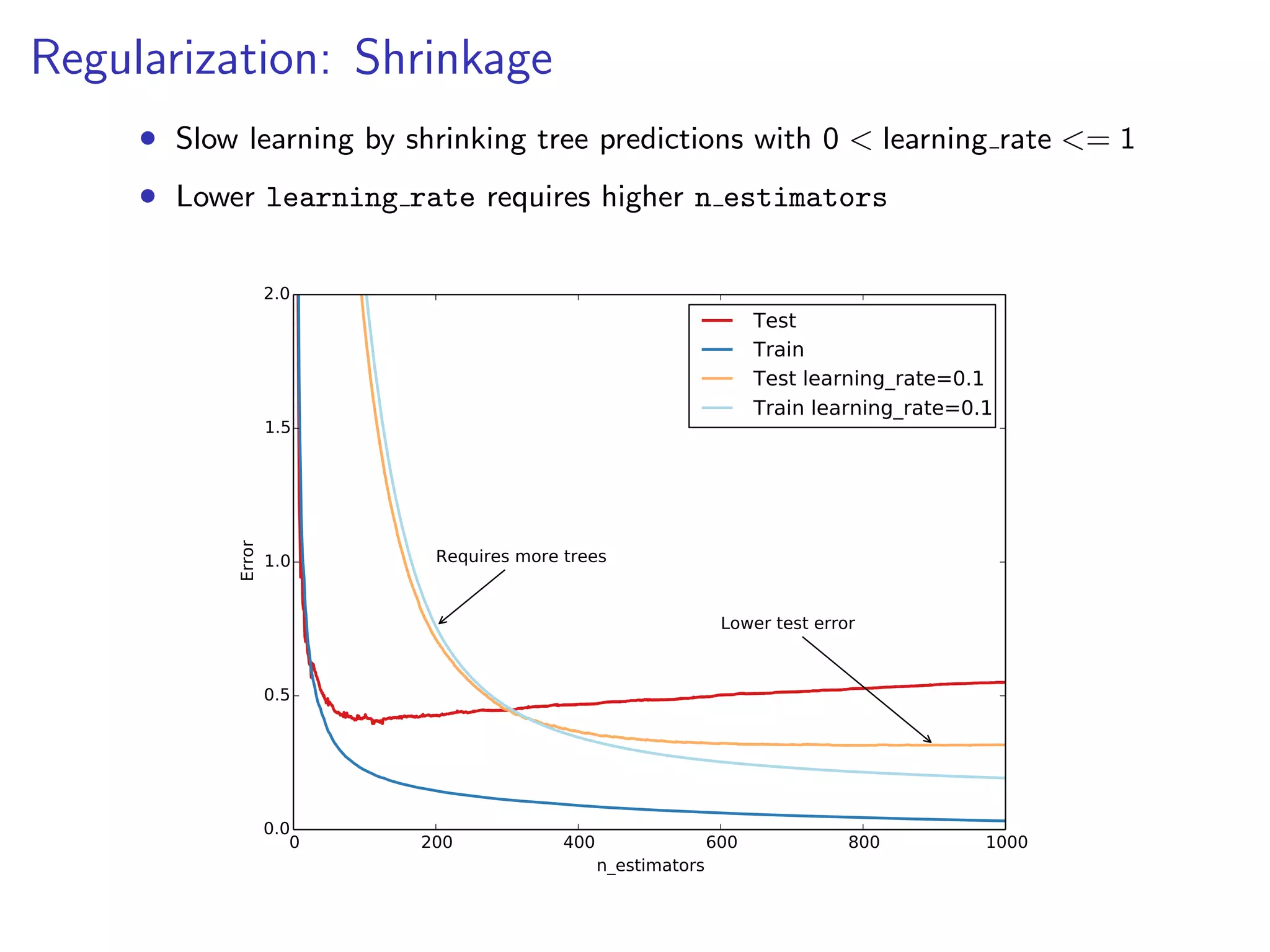
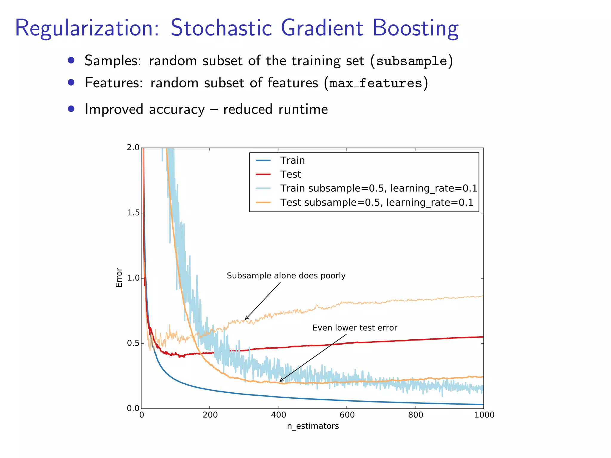
23. Model complexity & Overfitting
test_score = np.empty(len(est.estimators_))
for i, pred in enumerate(est.staged_predict(X_test)):
test_score[i] = est.loss_(y_test, pred)
plt.plot(np.arange(n_estimators) + 1, test_score, label=’Test’)
plt.plot(np.arange(n_estimators) + 1, est.train_score_, label=’Train’)
2.0
Test
Train
Regularization
1.5
GBRT provides a number of knobs to control
overfitting
Error
Lowest test
•1.0Tree structure error
• Shrinkage
• Stochastic Gradient Boosting
0.5
train-test gap
0.0
0
200
400
n_estimators
600
800
1000

24. Regularization: Tree structure
• The max depth of the trees controls the degree of features interactions
• Use min samples leaf to have a sufficient nr. of samples per leaf.

25. Regularization: Shrinkage
• Slow learning by shrinking tree predictions with 0 < learning rate <= 1
• Lower learning rate requires higher n estimators
2.0
Test
Train
Test learning_rate=0.1
Train learning_rate=0.1
Error
1.5
1.0
Requires more trees
Lower test error
0.5
0.0
0
200
400
n_estimators
600
800
1000

26. Regularization: Stochastic Gradient Boosting
• Samples: random subset of the training set (subsample)
• Features: random subset of features (max features)
• Improved accuracy – reduced runtime
2.0
Train
Test
Train subsample=0.5, learning_rate=0.1
Test subsample=0.5, learning_rate=0.1
Error
1.5
Subsample alone does poorly
1.0
Even lower test error
0.5
0.0
0
200
400
n_estimators
600
800
1000

27. Hyperparameter tuning
1. Set n estimators as high as possible (eg. 3000)
2. Tune hyperparameters via grid search.
from sklearn.grid_search import GridSearchCV
param_grid = {’learning_rate’: [0.1, 0.05, 0.02, 0.01],
’max_depth’: [4, 6],
’min_samples_leaf’: [3, 5, 9, 17],
’max_features’: [1.0, 0.3, 0.1]}
est = GradientBoostingRegressor(n_estimators=3000)
gs_cv = GridSearchCV(est, param_grid).fit(X, y)
# best hyperparameter setting
gs_cv.best_params_
3. Finally, set n estimators even higher and tune
learning rate.

28. Outline
1 Basics
2 Gradient Boosting
3 Gradient Boosting in Scikit-learn
4 Case Study: California housing

29. Case Study
California Housing dataset
• Predict log(medianHouseValue)
• Block groups in 1990 census
• 20.640 groups with 8 features
(median income, median age, lat,
lon, ...)
• Evaluation: Mean absolute error
on 80/20 split
Challenges
• Heterogeneous features
• Non-linear interactions

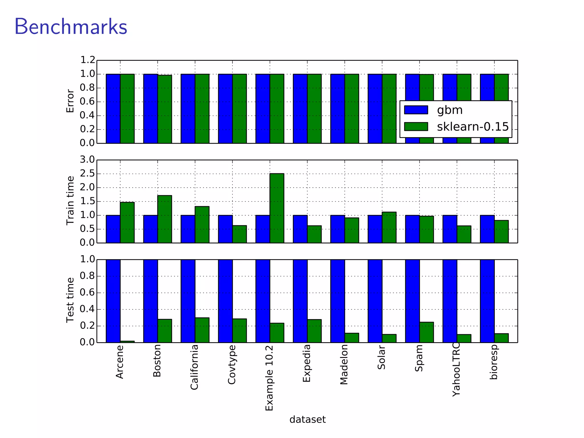
30. Predictive accuracy & runtime
Mean
Ridge
SVR
RF
GBRT
Train time [s]
0.006
28.0
26.3
192.0
Test time [ms]
0.11
2000.00
605.00
439.00
MAE
0.4635
0.2756
0.1888
0.1620
0.1438
0.5
Test
Train
0.4
error
0.3
0.2
0.1
0.0
0
500
1000
1500
n_estimators
2000
2500
3000

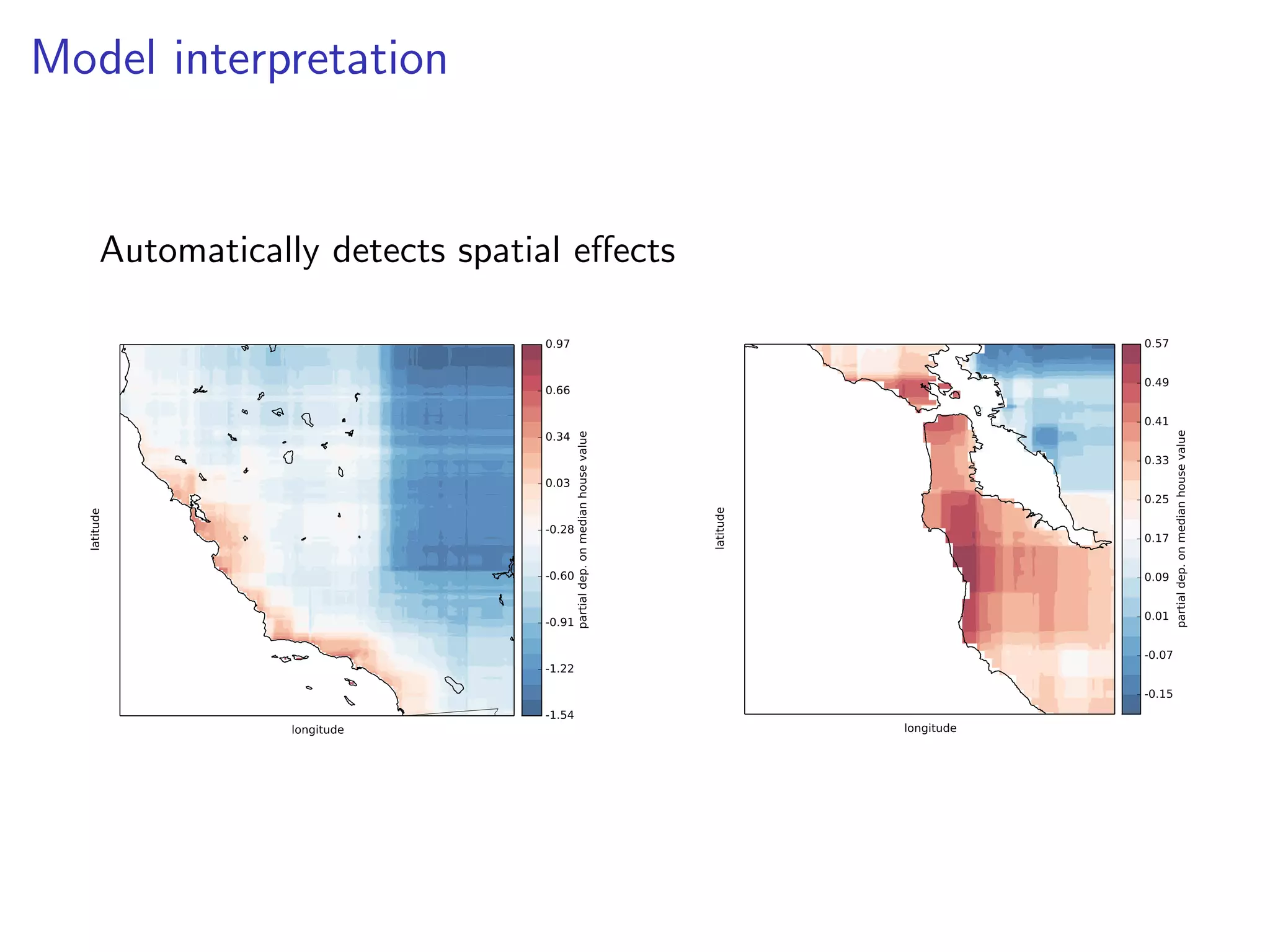
31. Model interpretation
Which features are important?
>>> est.feature_importances_
array([ 0.01, 0.38, ...])
MedInc
AveRooms
Longitude
AveOccup
Latitude
AveBedrms
Population
HouseAge
0.00
0.02
0.04
0.06
0.08 0.10 0.12
Relative importance
0.14
0.16
0.18

32. Model interpretation
What is the effect of a feature on the response?
from sklearn.ensemble import partial_dependence import as pd
Partial dependence
-0.12
0.09
0.2
3
0.02
0.16
-0.05
Partial dependence
Partial dependence of house value on nonlocation features
for the California housing dataset
0.6
0.6
0.4
0.4
0.2
0.2
0.0
0.0
0.2
0.2
0.4
0.4
1.5 3.0 4.5 6.0 7.5
2.0 2.5 3.0 3.5 4.0 4.5
10 20 30 40 50 60
MedInc
AveOccup
HouseAge
0.6
50
0.4
40
0.2
30
0.0
20
0.2
0.4
10
4 5 6 7 8
2.0 2.5 3.0 3.5 4.0
AveRooms
AveOccup
0.6
0.4
0.2
0.0
0.2
0.4
HouseAge
Partial dependence
Partial dependence
features = [’MedInc’, ’AveOccup’, ’HouseAge’, ’AveRooms’,
(’AveOccup’, ’HouseAge’)]
fig, axs = pd.plot_partial_dependence(est, X_train, features,
feature_names=names)

33. Model interpretation
Automatically detects spatial effects
0.97
0.57
0.66
0.49
0.41
partial dep. on median house value
partial dep. on median house value
0.34
0.33
-0.28
0.25
latitude
latitude
0.03
0.17
-0.60
0.09
-0.91
0.01
-0.07
-1.22
longitude
-1.54
-0.15
longitude

34. Summary
• Flexible non-parametric classification and regression technique
• Applicable to a variety of problems
• Solid, battle-worn implementation in scikit-learn

35. Thanks! Questions?

36. Test time
Train time
Error
1.2
1.0
0.8
0.6
0.4
0.2
0.0
3.0
2.5
2.0
1.5
1.0
0.5
0.0
1.0
0.8
0.6
0.4
0.2
0.0
dataset
bioresp
YahooLTRC
Spam
Solar
Madelon
Expedia
Example 10.2
Covtype
California
Boston
Arcene
Benchmarks
gbm
sklearn-0.15

37. Tipps & Tricks 1
Input layout
Use dtype=np.float32 to avoid memory copies and fortan layout for slight
runtime benefit.
X = np.asfortranarray(X, dtype=np.float32)

38. Tipps & Tricks 2
Feature interactions
GBRT automatically detects feature interactions but often explicit interactions
help.
Trees required to approximate X1 − X2 : 10 (left), 1000 (right).
0.3
1.0
0.2
x-y
0.0
0.0
0.1
0.5
0.2
1.0
0.8
0.6
x
0.4
0.2
0.0 1.0
0.8
0.6
0.4
y
0.2
x-y
0.5
0.1
0.3
0.0
1.0
0.8
0.6
x
0.4
0.2
0.0 1.0
0.8
0.6
0.4
y
0.2
1.0
0.0

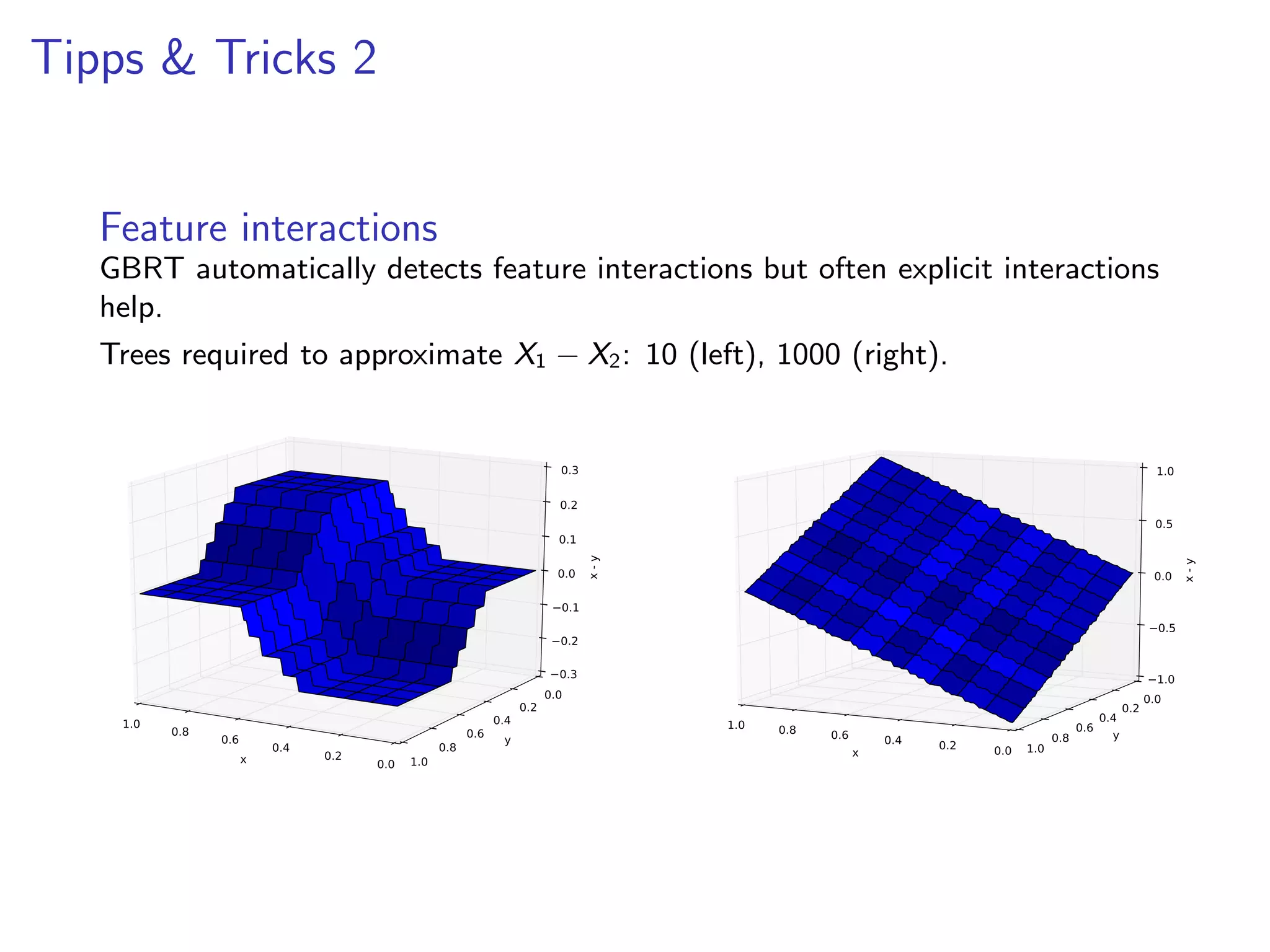
39. Tipps & Tricks 3
Categorical variables
Sklearn requires that categorical variables are encoded as numerics. Tree-based
methods work well with ordinal encoding:
df = pd.DataFrame(data={’icao’: [’CRJ2’, ’A380’, ’B737’, ’B737’]})
# ordinal encoding
df_enc = pd.DataFrame(data={’icao’: np.unique(df.icao,
return_inverse=True)[1]})
X = np.asfortranarray(df_enc.values, dtype=np.float32)