Downloaded 65 times
![“ [Statistics are] the only tools by which an opening can be cut through the formidable thicket of difficulties that bars the path of those who pursue the Science of Man.” [Sir] Francis Galton (1822-1911)](https://image.slidesharecdn.com/statisticsexcellent-110131035957-phpapp02/85/Statistics-excellent-2-320.jpg)

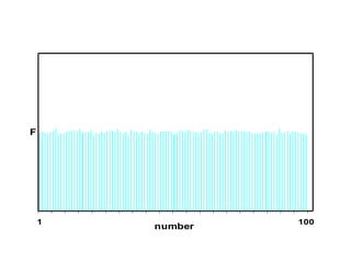
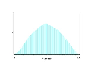
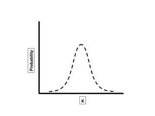

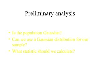
![[On the Gaussian curve] “Experimentalists think that it is a mathematical theorem while the mathematicians believe it to be an experimental fact.” Gabriel Lippman (1845-1921 )](https://image.slidesharecdn.com/statisticsexcellent-110131035957-phpapp02/85/Statistics-excellent-71-320.jpg)
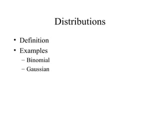
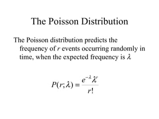
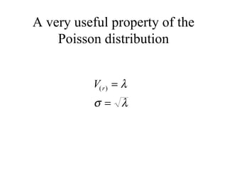
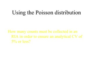
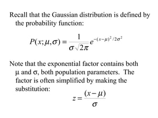
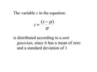
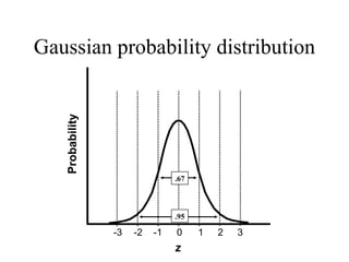
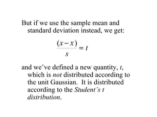
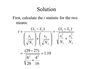
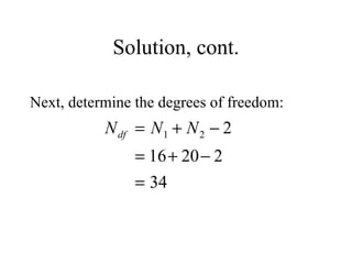
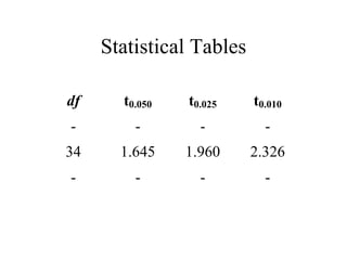
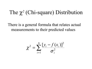
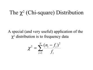


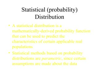
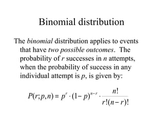
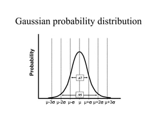
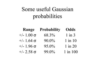
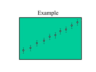
This document discusses various statistical concepts and their applications in clinical laboratories. It defines descriptive statistics, statistical analysis, measures of central tendency (mean, median, mode), measures of variation (variance, standard deviation), probability distributions (binomial, Gaussian, Poisson), and statistical tests (t-test, chi-square, F-test). It provides examples of how these statistical methods are used to monitor laboratory test performance, interpret results, and compare different laboratory instruments and methods.