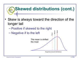
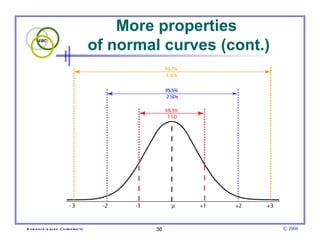
Biostatistics Basics   An introduction to an expansive and complex field
Common statistical terms  Data  Measurements or observations of a variable Variable  A characteristic that is observed or manipulated  Can take on different values
Statistical terms (cont.)  Independent variables  Precede dependent variables in time  Are often manipulated by the researcher The treatment or intervention that is used in a study Dependent variables  What is measured as an outcome in a study  Values depend on the independent variable
Statistical terms (cont.) Parameters Summary data from a population Statistics Summary data from a sample
Populations A population is the group from which a sample is drawn  e.g., headache patients in a chiropractic office; automobile crash victims in an emergency room  In research, it is not practical to include all members of a population Thus, a sample (a subset of a population) is taken
Random samples  Subjects are selected from a population so that each individual has an equal chance of being selected  Random samples are representative of the source population  Non-random samples are not representative May be biased regarding age, severity of the condition, socioeconomic status etc.
Random samples (cont.) Random samples are rarely utilized in health care research Instead, patients are randomly assigned to treatment and control groups  Each person has an equal chance of being assigned to either of the groups  Random assignment is also known as randomization
Descriptive statistics ( DSs) A way to summarize data from a sample or a population  DSs illustrate the  shape ,  central tendency , and  variability  of a set of data  The shape of data has to do with the frequencies of the values of observations
DSs (cont.) Central tendency describes the location of the middle of the data  Variability is the extent values are spread above and below the middle values a.k.a., Dispersion DSs can be distinguished from inferential statistics  DSs are not capable of testing hypotheses
Hypothetical study data (partial from book) Case #  Visits 1 7 2 2  3 2  4 3  5 4  6 3  7 5  8 3  9 4  10 6  11 2  12 3  13 7  14 4  Distribution provides a summary of: Frequencies of each of the values  2 –  3 3 –  4   4 –  3   5 –  1 6 –  1 7 –  2 Ranges of values  Lowest =  2 Highest =  7 etc.
Frequency distribution table Frequency     Percent Cumulative % 2   3   21.4 21.4 3   4   28.6 50.0  4   3     21.4 71.4 5   1   7.1 78.5 6   1   7.1 85.6 7   2   14.3   100.0
Frequency distributions are  often depicted by a histogram
Histograms (cont.) A histogram is a type of bar chart, but there are no spaces between the bars Histograms are used to visually depict frequency distributions of continuous data Bar charts are used to depict categorical information  e.g., Male–Female, Mild–Moderate–Severe, etc.
Measures of central tendency Mean (a.k.a.,  average )  The most commonly used DS To calculate the mean Add all values of a series of numbers and then divided by the total number of elements
Formula to calculate the mean Mean of a sample Mean of a population  (X bar) refers to the mean of a sample and  refers to the mean of a population  X  is a command that adds all of the  X  values  n  is the total number of values in the series of a sample and  N  is the same for a population
Measures of central  tendency (cont.) Mode  The most frequently  occurring value in a  series The modal value is  the highest bar in a  histogram Mode
Measures of central  tendency (cont.) Median The value that divides a series of values in half when they are all listed in order  When there are an odd number of values  The median is the middle value  When there are an even number of values Count from each end of the series toward the middle and then average the 2 middle values
Measures of central  tendency (cont.) Each of the three methods of measuring central tendency has certain advantages and disadvantages Which method should be used? It depends on the type of data that is being analyzed  e.g., categorical, continuous, and the level of measurement that is involved
Levels of measurement There are 4 levels of measurement  Nominal, ordinal, interval, and ratio Nominal  Data are coded by a number, name, or letter that is assigned to a category or group  Examples Gender (e.g., male, female)  Treatment preference (e.g., manipulation, mobilization, massage)
Levels of measurement (cont.) Ordinal  Is similar to nominal because the measurements involve categories However, the categories are ordered by rank Examples Pain level (e.g., mild, moderate, severe)  Military rank (e.g., lieutenant, captain, major, colonel, general)
Levels of measurement (cont.) Ordinal values only describe order, not quantity Thus, severe pain is not the same as 2 times mild pain The only mathematical operations allowed for nominal and ordinal data are counting of categories e.g., 25 males and 30 females
Levels of measurement (cont.) Interval  Measurements are ordered (like ordinal data)  Have equal intervals  Does not have a true zero  Examples The Fahrenheit scale, where 0° does not correspond to an absence of heat (no true zero)  In contrast to Kelvin, which does have a true zero
Levels of measurement (cont.) Ratio  Measurements have equal intervals  There is a true zero  Ratio is the most advanced level of measurement, which can handle most types of mathematical operations
Levels of measurement (cont.) Ratio examples Range of motion  No movement corresponds to zero degrees The interval between 10 and 20 degrees is the same as between 40 and 50 degrees  Lifting capacity A person who is unable to lift scores zero A person who lifts 30 kg can lift twice as much as one who lifts 15 kg
Levels of measurement (cont.) NOIR is a mnemonic to help remember the names and order of the levels of measurement N ominal O rdinal I nterval R atio
Levels of measurement (cont.) Symmetrical – Mean Skewed – Median Addition, subtraction, multiplication and division  Ratio Symmetrical – Mean Skewed – Median Addition and subtraction Interval Median Greater or less than  operations Ordinal Mode Counting Nominal Best measure of central tendency Permissible mathematic operations Measurement scale
The shape of data  Histograms of frequency distributions have shape Distributions are often symmetrical with most scores falling in the middle and fewer toward the extremes Most biological data are symmetrically distributed and form a  normal   curve  (a.k.a, bell-shaped curve)
The shape of data (cont.)  Line depicting the  shape  of the data
The normal distribution The area under a normal curve has a  normal distribution  (a.k.a., Gaussian distribution)  Properties of a normal distribution It is symmetric about its mean The highest point is at its mean The height of the curve decreases as one moves away from the mean in either direction, approaching, but never reaching zero
The normal distribution (cont.)  Mean A normal distribution is symmetric about its mean As one moves away from  the mean in either direction  the height of the curve  decreases, approaching,  but never reaching zero The highest point of the overlying  normal curve is at the mean
The normal distribution (cont.)  Mean = Median = Mode
Skewed distributions The data are not distributed symmetrically in skewed distributions  Consequently, the mean, median, and mode are not equal and are in different positions Scores are clustered at one end of the distribution A small number of extreme values are located in the limits of the opposite end
Skewed distributions (cont.) Skew is always toward the direction of the longer tail Positive if skewed to the right Negative if to the left The mean is shifted  the most
Skewed distributions (cont.) Because the mean is shifted so much, it is not the best estimate of the average score for skewed distributions The median is a better estimate of the center of skewed distributions It will be the central point of any distribution 50% of the values are above and 50% below the median
More properties  of normal curves About 68.3% of the area under a normal curve is within one standard deviation (SD) of the mean About 95.5% is within two SDs About 99.7% is within three SDs
More properties  of normal curves (cont.)
Standard deviation (SD)  SD is a measure of the variability of a set of data  The mean represents the average of a group of scores, with some of the scores being above the mean and some below  This range of scores is referred to as  variability  or  spread   Variance  ( S 2 ) is another measure of spread
SD (cont.) In effect, SD is the average amount of spread in a distribution of scores The next slide is a group of 10 patients whose mean age is 40 years  Some are older than 40 and some younger
SD (cont.) Ages are spread  out along an X axis  The amount ages are  spread out is known as  dispersion  or  spread
Distances ages deviate above and below the mean  Adding deviations  always equals zero   Etc.
Calculating  S 2 To find the average, one would normally total the scores above and below the mean, add them together, and then divide by the number of values However, the total always equals zero Values must first be squared, which cancels the negative signs
Calculating  S 2  cont.  Symbol for SD of a sample     for a population  S 2  is not in the  same units (age),  but SD is
Calculating SD with Excel Enter values in a column
SD with Excel (cont.) Click  Data Analysis   on the  Tools  menu
SD with Excel (cont.) Select  Descriptive Statistics  and click OK
SD with Excel (cont.) Click  Input Range  icon
SD with Excel (cont.) Highlight all the values in the column
SD with Excel (cont.) Check if labels are  in the first row Check  Summary Statistics Click OK
SD with Excel (cont.) SD is calculated precisely Plus several other DSs
Wide spread results in higher SDs narrow spread in lower SDs
Spread is important when comparing 2 or more group means  It is more difficult to  see a clear distinction between groups  in the upper example  because the spread is  wider, even though the  means are the same
z-scores The number of SDs that a specific score is above or below the mean in a distribution  Raw scores can be converted to z-scores by subtracting the mean from the raw score then dividing the difference by the SD
z-scores (cont.) Standardization  The process of converting raw to z-scores  The resulting distribution of z-scores will always have a mean of zero, a SD of one, and an area under the curve equal to one The proportion of scores that are higher or lower than a specific z-score can be determined by referring to a z-table
z-scores (cont.) Refer to a z-table to find proportion under the curve
z-scores (cont.) 0.9332 Corresponds to the area  under the curve in black 0.9441 0.9429 0.9418 0.9406 0.9394 0.9382 0.9370 0.9357 0.9345 0.9332 1.5 0.9319 0.9306 0.9292 0.9279 0.9265 0.9251 0.9236 0.9222 0.9207 0.9192 1.4 0.9177 0.9162 0.9147 0.9131 0.9115 0.9099 0.9082 0.9066 0.9049 0.9032 1.3 0.9015 0.8997 0.8980 0.8962 0.8944 0.8925 0.8907 0.8888 0.8869 0.8849 1.2 0.8830 0.8810 0.8790 0.8770 0.8749 0.8729 0.8708 0.8686 0.8665 0.8643 1.1 0.8621 0.8599 0.8577 0.8554 0.8531 0.8508 0.8485 0.8461 0.8438 0.8413 1.0 0.8389 0.8365 0.8340 0.8315 0.8289 0.8264 0.8238 0.8212 0.8186 0.8159 0.9 0.8133 0.8106 0.8078 0.8051 0.8023 0.7995 0.7967 0.7939 0.7910 0.7881 0.8 0.7852 0.7823 0.7794 0.7764 0.7734 0.7704 0.7673 0.7642 0.7611 0.7580 0.7 0.7549 0.7517 0.7486 0.7454 0.7422 0.7389 0.7357 0.7324 0.7291 0.7257 0.6 0.7224 0.7190 0.7157 0.7123 0.7088 0.7054 0.7019 0.6985 0.6950 0.6915 0.5 0.6879 0.6844 0.6808 0.6772 0.6736 0.6700 0.6664 0.6628 0.6591 0.6554 0.4 0.6517 0.6480 0.6443 0.6406 0.6368 0.6331 0.6293 0.6255 0.6217 0.6179 0.3 0.6141 0.6103 0.6064 0.6026 0.5987 0.5948 0.5910 0.5871 0.5832 0.5793 0.2 0.5753 0.5714 0.5675 0.5636 0.5596 0.5557 0.5517 0.5478 0.5438 0.5398 0.1 0.5359 0.5319 0.5279 0.5239 0.5199 0.5160 0.5120 0.5080 0.5040 0.5000 0.0 0.09 0.08 0.07 0.06 0.05 0.04 0.03 0.02 0.01 0.00 Z   Partial z-table (to z = 1.5) showing proportions of the  area under a normal curve for different values of z.

Biostatistics basics-biostatistics4734

  • 1.
    Biostatistics Basics An introduction to an expansive and complex field
  • 2.
    Common statistical terms Data Measurements or observations of a variable Variable A characteristic that is observed or manipulated Can take on different values
  • 3.
    Statistical terms (cont.) Independent variables Precede dependent variables in time Are often manipulated by the researcher The treatment or intervention that is used in a study Dependent variables What is measured as an outcome in a study Values depend on the independent variable
  • 4.
    Statistical terms (cont.)Parameters Summary data from a population Statistics Summary data from a sample
  • 5.
    Populations A populationis the group from which a sample is drawn e.g., headache patients in a chiropractic office; automobile crash victims in an emergency room In research, it is not practical to include all members of a population Thus, a sample (a subset of a population) is taken
  • 6.
    Random samples Subjects are selected from a population so that each individual has an equal chance of being selected Random samples are representative of the source population Non-random samples are not representative May be biased regarding age, severity of the condition, socioeconomic status etc.
  • 7.
    Random samples (cont.)Random samples are rarely utilized in health care research Instead, patients are randomly assigned to treatment and control groups Each person has an equal chance of being assigned to either of the groups Random assignment is also known as randomization
  • 8.
    Descriptive statistics (DSs) A way to summarize data from a sample or a population DSs illustrate the shape , central tendency , and variability of a set of data The shape of data has to do with the frequencies of the values of observations
  • 9.
    DSs (cont.) Centraltendency describes the location of the middle of the data Variability is the extent values are spread above and below the middle values a.k.a., Dispersion DSs can be distinguished from inferential statistics DSs are not capable of testing hypotheses
  • 10.
    Hypothetical study data(partial from book) Case # Visits 1 7 2 2 3 2 4 3 5 4 6 3 7 5 8 3 9 4 10 6 11 2 12 3 13 7 14 4 Distribution provides a summary of: Frequencies of each of the values 2 – 3 3 – 4 4 – 3 5 – 1 6 – 1 7 – 2 Ranges of values Lowest = 2 Highest = 7 etc.
  • 11.
    Frequency distribution tableFrequency Percent Cumulative % 2 3 21.4 21.4 3 4 28.6 50.0 4 3 21.4 71.4 5 1 7.1 78.5 6 1 7.1 85.6 7 2 14.3 100.0
  • 12.
    Frequency distributions are often depicted by a histogram
  • 13.
    Histograms (cont.) Ahistogram is a type of bar chart, but there are no spaces between the bars Histograms are used to visually depict frequency distributions of continuous data Bar charts are used to depict categorical information e.g., Male–Female, Mild–Moderate–Severe, etc.
  • 14.
    Measures of centraltendency Mean (a.k.a., average ) The most commonly used DS To calculate the mean Add all values of a series of numbers and then divided by the total number of elements
  • 15.
    Formula to calculatethe mean Mean of a sample Mean of a population (X bar) refers to the mean of a sample and refers to the mean of a population  X is a command that adds all of the X values n is the total number of values in the series of a sample and N is the same for a population
  • 16.
    Measures of central tendency (cont.) Mode The most frequently occurring value in a series The modal value is the highest bar in a histogram Mode
  • 17.
    Measures of central tendency (cont.) Median The value that divides a series of values in half when they are all listed in order When there are an odd number of values The median is the middle value When there are an even number of values Count from each end of the series toward the middle and then average the 2 middle values
  • 18.
    Measures of central tendency (cont.) Each of the three methods of measuring central tendency has certain advantages and disadvantages Which method should be used? It depends on the type of data that is being analyzed e.g., categorical, continuous, and the level of measurement that is involved
  • 19.
    Levels of measurementThere are 4 levels of measurement Nominal, ordinal, interval, and ratio Nominal Data are coded by a number, name, or letter that is assigned to a category or group Examples Gender (e.g., male, female) Treatment preference (e.g., manipulation, mobilization, massage)
  • 20.
    Levels of measurement(cont.) Ordinal Is similar to nominal because the measurements involve categories However, the categories are ordered by rank Examples Pain level (e.g., mild, moderate, severe) Military rank (e.g., lieutenant, captain, major, colonel, general)
  • 21.
    Levels of measurement(cont.) Ordinal values only describe order, not quantity Thus, severe pain is not the same as 2 times mild pain The only mathematical operations allowed for nominal and ordinal data are counting of categories e.g., 25 males and 30 females
  • 22.
    Levels of measurement(cont.) Interval Measurements are ordered (like ordinal data) Have equal intervals Does not have a true zero Examples The Fahrenheit scale, where 0° does not correspond to an absence of heat (no true zero) In contrast to Kelvin, which does have a true zero
  • 23.
    Levels of measurement(cont.) Ratio Measurements have equal intervals There is a true zero Ratio is the most advanced level of measurement, which can handle most types of mathematical operations
  • 24.
    Levels of measurement(cont.) Ratio examples Range of motion No movement corresponds to zero degrees The interval between 10 and 20 degrees is the same as between 40 and 50 degrees Lifting capacity A person who is unable to lift scores zero A person who lifts 30 kg can lift twice as much as one who lifts 15 kg
  • 25.
    Levels of measurement(cont.) NOIR is a mnemonic to help remember the names and order of the levels of measurement N ominal O rdinal I nterval R atio
  • 26.
    Levels of measurement(cont.) Symmetrical – Mean Skewed – Median Addition, subtraction, multiplication and division Ratio Symmetrical – Mean Skewed – Median Addition and subtraction Interval Median Greater or less than operations Ordinal Mode Counting Nominal Best measure of central tendency Permissible mathematic operations Measurement scale
  • 27.
    The shape ofdata Histograms of frequency distributions have shape Distributions are often symmetrical with most scores falling in the middle and fewer toward the extremes Most biological data are symmetrically distributed and form a normal curve (a.k.a, bell-shaped curve)
  • 28.
    The shape ofdata (cont.) Line depicting the shape of the data
  • 29.
    The normal distributionThe area under a normal curve has a normal distribution (a.k.a., Gaussian distribution) Properties of a normal distribution It is symmetric about its mean The highest point is at its mean The height of the curve decreases as one moves away from the mean in either direction, approaching, but never reaching zero
  • 30.
    The normal distribution(cont.) Mean A normal distribution is symmetric about its mean As one moves away from the mean in either direction the height of the curve decreases, approaching, but never reaching zero The highest point of the overlying normal curve is at the mean
  • 31.
    The normal distribution(cont.) Mean = Median = Mode
  • 32.
    Skewed distributions Thedata are not distributed symmetrically in skewed distributions Consequently, the mean, median, and mode are not equal and are in different positions Scores are clustered at one end of the distribution A small number of extreme values are located in the limits of the opposite end
  • 33.
    Skewed distributions (cont.)Skew is always toward the direction of the longer tail Positive if skewed to the right Negative if to the left The mean is shifted the most
  • 34.
    Skewed distributions (cont.)Because the mean is shifted so much, it is not the best estimate of the average score for skewed distributions The median is a better estimate of the center of skewed distributions It will be the central point of any distribution 50% of the values are above and 50% below the median
  • 35.
    More properties of normal curves About 68.3% of the area under a normal curve is within one standard deviation (SD) of the mean About 95.5% is within two SDs About 99.7% is within three SDs
  • 36.
    More properties of normal curves (cont.)
  • 37.
    Standard deviation (SD) SD is a measure of the variability of a set of data The mean represents the average of a group of scores, with some of the scores being above the mean and some below This range of scores is referred to as variability or spread Variance ( S 2 ) is another measure of spread
  • 38.
    SD (cont.) Ineffect, SD is the average amount of spread in a distribution of scores The next slide is a group of 10 patients whose mean age is 40 years Some are older than 40 and some younger
  • 39.
    SD (cont.) Agesare spread out along an X axis The amount ages are spread out is known as dispersion or spread
  • 40.
    Distances ages deviateabove and below the mean Adding deviations always equals zero Etc.
  • 41.
    Calculating S2 To find the average, one would normally total the scores above and below the mean, add them together, and then divide by the number of values However, the total always equals zero Values must first be squared, which cancels the negative signs
  • 42.
    Calculating S2 cont. Symbol for SD of a sample  for a population S 2 is not in the same units (age), but SD is
  • 43.
    Calculating SD withExcel Enter values in a column
  • 44.
    SD with Excel(cont.) Click Data Analysis on the Tools menu
  • 45.
    SD with Excel(cont.) Select Descriptive Statistics and click OK
  • 46.
    SD with Excel(cont.) Click Input Range icon
  • 47.
    SD with Excel(cont.) Highlight all the values in the column
  • 48.
    SD with Excel(cont.) Check if labels are in the first row Check Summary Statistics Click OK
  • 49.
    SD with Excel(cont.) SD is calculated precisely Plus several other DSs
  • 50.
    Wide spread resultsin higher SDs narrow spread in lower SDs
  • 51.
    Spread is importantwhen comparing 2 or more group means It is more difficult to see a clear distinction between groups in the upper example because the spread is wider, even though the means are the same
  • 52.
    z-scores The numberof SDs that a specific score is above or below the mean in a distribution Raw scores can be converted to z-scores by subtracting the mean from the raw score then dividing the difference by the SD
  • 53.
    z-scores (cont.) Standardization The process of converting raw to z-scores The resulting distribution of z-scores will always have a mean of zero, a SD of one, and an area under the curve equal to one The proportion of scores that are higher or lower than a specific z-score can be determined by referring to a z-table
  • 54.
    z-scores (cont.) Referto a z-table to find proportion under the curve
  • 55.
    z-scores (cont.) 0.9332Corresponds to the area under the curve in black 0.9441 0.9429 0.9418 0.9406 0.9394 0.9382 0.9370 0.9357 0.9345 0.9332 1.5 0.9319 0.9306 0.9292 0.9279 0.9265 0.9251 0.9236 0.9222 0.9207 0.9192 1.4 0.9177 0.9162 0.9147 0.9131 0.9115 0.9099 0.9082 0.9066 0.9049 0.9032 1.3 0.9015 0.8997 0.8980 0.8962 0.8944 0.8925 0.8907 0.8888 0.8869 0.8849 1.2 0.8830 0.8810 0.8790 0.8770 0.8749 0.8729 0.8708 0.8686 0.8665 0.8643 1.1 0.8621 0.8599 0.8577 0.8554 0.8531 0.8508 0.8485 0.8461 0.8438 0.8413 1.0 0.8389 0.8365 0.8340 0.8315 0.8289 0.8264 0.8238 0.8212 0.8186 0.8159 0.9 0.8133 0.8106 0.8078 0.8051 0.8023 0.7995 0.7967 0.7939 0.7910 0.7881 0.8 0.7852 0.7823 0.7794 0.7764 0.7734 0.7704 0.7673 0.7642 0.7611 0.7580 0.7 0.7549 0.7517 0.7486 0.7454 0.7422 0.7389 0.7357 0.7324 0.7291 0.7257 0.6 0.7224 0.7190 0.7157 0.7123 0.7088 0.7054 0.7019 0.6985 0.6950 0.6915 0.5 0.6879 0.6844 0.6808 0.6772 0.6736 0.6700 0.6664 0.6628 0.6591 0.6554 0.4 0.6517 0.6480 0.6443 0.6406 0.6368 0.6331 0.6293 0.6255 0.6217 0.6179 0.3 0.6141 0.6103 0.6064 0.6026 0.5987 0.5948 0.5910 0.5871 0.5832 0.5793 0.2 0.5753 0.5714 0.5675 0.5636 0.5596 0.5557 0.5517 0.5478 0.5438 0.5398 0.1 0.5359 0.5319 0.5279 0.5239 0.5199 0.5160 0.5120 0.5080 0.5040 0.5000 0.0 0.09 0.08 0.07 0.06 0.05 0.04 0.03 0.02 0.01 0.00 Z Partial z-table (to z = 1.5) showing proportions of the area under a normal curve for different values of z.