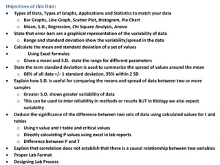
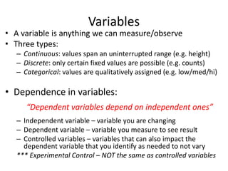
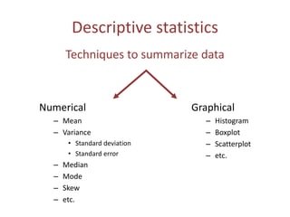
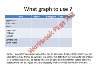
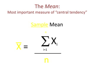
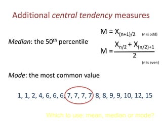
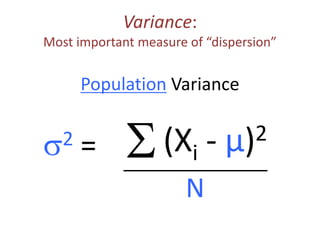
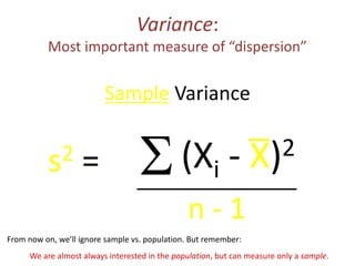
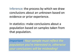
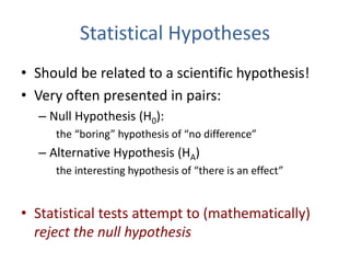
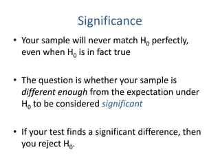
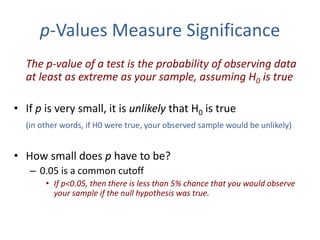
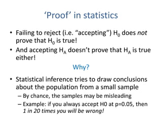
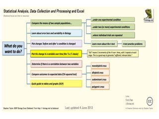
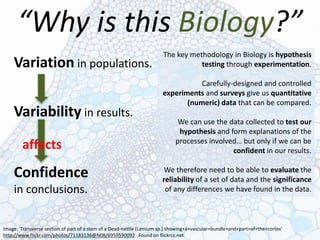
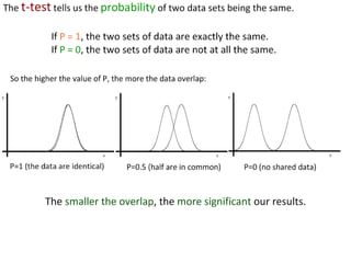
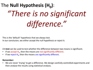
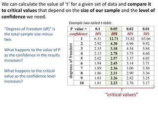
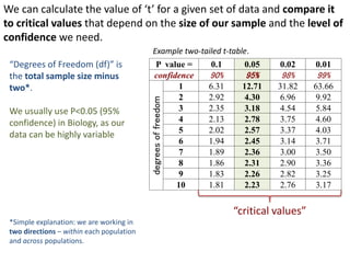
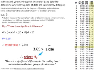
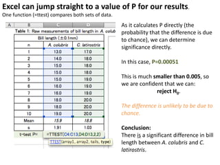
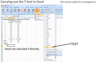
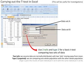
SlideShare a Scribd company logo
Statistical Analysis
IB Diploma Biology
Objectives of this Unit:
 Types of Data, Types of Graphs, Applications and Statistics to match your data
o Bar Graphs, Line Graph, Scatter Plot, Histogram, Pie Chart
o Mean, S.D., Regression, Chi Square Analysis, Anova
 State that error bars are a graphical representation of the variability of data
o Range and standard deviation show the variability/spread in the data
 Calculate the mean and standard deviation of a set of values
 Using Excel formulas
o Given a mean and S.D. state the range for different parameters
 State the term standard deviation is used to summarize the spread of values around the mean
o 68% of all data +/- 1 standard deviation, 95% within 2 SD
 Explain how S.D. is useful for comparing the means and spread of data between two or more
samples
o Greater S.D. shows greater variability of data
o This can be used to inter reliability in methods or results BUT in Biology we also expect
variability
 Deduce the significance of the difference between two sets of data using calculated values for t and
tables
o Using t value and t table and critical values
o Directly calculating P values using excel in lab reports
o Difference between P and T
 Explain that correlation does not establish that there is a causal relationship between two variables
 Proper Lab Format
 Designing Lab Process
What are statistics?
• Statistics are numbers used to:
Describe and draw conclusions about DATA
• These are called descriptive (or “univariate”) and
inferential (or “analytical”) statistics, respectively.
Variables
• A variable is anything we can measure/observe
• Three types:
– Continuous: values span an uninterrupted range (e.g. height)
– Discrete: only certain fixed values are possible (e.g. counts)
– Categorical: values are qualitatively assigned (e.g. low/med/hi)
• Dependence in variables:
“Dependent variables depend on independent ones”
– Independent variable – variable you are changing
– Dependent variable – variable you measure to see result
– Controlled variables – variables that can also impact the
dependent variable that you identify as needed to not vary
*** Experimental Control – NOT the same as controlled variables
Descriptive statistics
Numerical
– Mean
– Variance
• Standard deviation
• Standard error
– Median
– Mode
– Skew
– etc.
Graphical
– Histogram
– Boxplot
– Scatterplot
– etc.
Techniques to summarize data
Graphic Applications
What graph to use ?
Line Scatter Histogram Bar
Appropriat
e for data
when:
Important
Features
Include
Sample and
other notes
Outlier - An outlier is an observation that lies an abnormal distance from other values in
a random sample from a population. In a sense, this definition leaves it up to the analyst
(or a consensus process) to decide what will be considered abnormal. Before abnormal
observations can be singled out, it is necessary to characterize normal observations.
Numeric Descriptive Statistics
S
The Mean:
Most important measure of “central tendency”
Xi
i=1
N
m =
N
Population Mean
S
The Mean:
Most important measure of “central tendency”
i=1
n
n
Sample Mean
X =
Xi
Additional central tendency measures
M = X(n+1)/2 (n is odd)
Median: the 50th percentile
(n is even)
Xn/2 + X(n/2)+1
2
M =
Mode: the most common value
1, 1, 2, 4, 6, 6, 6, 7, 7, 7, 7, 8, 8, 9, 9, 10, 12, 15
Which to use: mean, median or mode?
Variance:
Most important measure of “dispersion”
s2 = S
N
Population Variance
(Xi - µ)2
Variance:
Most important measure of “dispersion”
s2 = S
n - 1
Sample Variance
(Xi - X)2
From now on, we’ll ignore sample vs. population. But remember:
We are almost always interested in the population, but can measure only a sample.
“Graphical Statistics”
Lets look deeper into graphs now
The Friendly Histogram
• Histograms represent the distribution of data
• They allow you to visualize the mean, median,
mode, variance, and skew at once!
Constructing a Histogram is Easy
X (data)
7.4
7.6
8.4
8.9
10.0
10.3
11.5
11.5
12.0
12.3
Histogram of X
Value
6 8 10 12 14
0
1
2
3
Frequency
(count)
Interpreting Histograms
• Mean?
• Median?
• Mode?
• Standard
deviation?
• Variance?
• Skew?
(which way does the
“tail” point?)
• Shape?
Value
0 20 40 60
0
20
40
Frequency
Interpreting Histograms
• Mean?
= 9.2
• Median? = 6.5
• Mode?
= 3
• Standard
deviation? = 8.3
• Variance?
• Skew?
(which way does the
“tail” point?)
• Shape?
Value
0 20 40 60
0
20
40
Frequency
An alternative:
Boxplots
0 20 40
0
20
40
Value
Frequency
Boxplots also
summarize a lot
of information...
Within each sample:
6
5
4
3
2
1
SC Ba Se Es Da Is Fe
Island
Weight(kg)
Compared across samples:
25% percentile
75% percentile
Median
“Outliers”
Normality
The Normal Distribution
aka “Gaussian” distribution
• Occurs frequently in nature
• Especially for measures that
are based on sums, such as:
– sample means
– body weight
– “error”
• Many statistics are based on
the assumption of normality
– You must make sure your data
are normal, or try something
else!
Sample normal data:
Histogram + theoretical distribution
(i.e. sample vs. population)
Properties of the Normal Distribution
• Symmetric
Mean = Median = Mode
• Theoretical percentiles can be computed exactly
~68% of data are within 1 standard deviation of the mean
>99% within 3 s.d.
“skinny tails”
>99%
~95%
~68%
Important!
Handy!
Amazing!
What if my data aren’t Normal?
• It’s OK!
• Although lots of data are Gaussian (because of the CLT),
many simply aren’t.
– Example: Fire return intervals
Time between fires (yr)
• Solutions:
– Transform data to make it
normal (e.g. take logs)
– Use a test that doesn’t
assume normal data
• Don’t worry, there are plenty
• Especially these days...
• Many stats work OK as long as data are “reasonably” normal
Break!
Inferential Statistics:
Day 2
Inference: the process by which we draw
conclusions about an unknown based on
evidence or prior experience.
In statistics: make conclusions about a
population based on samples taken from
that population.
Important: Your sample must reflect the
population you’re interested in, otherwise
your conclusions will be misleading!
Statistical Hypotheses
• Should be related to a scientific hypothesis!
• Very often presented in pairs:
– Null Hypothesis (H0):
the “boring” hypothesis of “no difference”
– Alternative Hypothesis (HA)
the interesting hypothesis of “there is an effect”
• Statistical tests attempt to (mathematically)
reject the null hypothesis
Significance
• Your sample will never match H0 perfectly,
even when H0 is in fact true
• The question is whether your sample is
different enough from the expectation under
H0 to be considered significant
• If your test finds a significant difference, then
you reject H0.
p-Values Measure Significance
The p-value of a test is the probability of observing data
at least as extreme as your sample, assuming H0 is true
• If p is very small, it is unlikely that H0 is true
(in other words, if H0 were true, your observed sample would be unlikely)
• How small does p have to be?
– 0.05 is a common cutoff
• If p<0.05, then there is less than 5% chance that you would observe
your sample if the null hypothesis was true.
‘Proof’ in statistics
• Failing to reject (i.e. “accepting”) H0 does not
prove that H0 is true!
• And accepting HA doesn’t prove that HA is true
either!
Why?
• Statistical inference tries to draw conclusions
about the population from a small sample
– By chance, the samples may be misleading
– Example: if you always accept H0 at p=0.05, then
1 in 20 times you will be wrong!
Play it Safe
Avoid using the term Prove in your labs
Instead say “the data accepts or supports” the
hypothesis
Watch out for reaching – classic student error,
stick to the scope of your lab data in your
conclusions, this is not your life work.
“Why is this Biology?”
Variation in populations.
Variability in results.
affects
Confidence
in conclusions.
The key methodology in Biology is hypothesis
testing through experimentation.
Carefully-designed and controlled
experiments and surveys give us quantitative
(numeric) data that can be compared.
We can use the data collected to test our
hypothesis and form explanations of the
processes involved… but only if we can be
confident in our results.
We therefore need to be able to evaluate the
reliability of a set of data and the significance
of any differences we have found in the data.
Image: 'Transverse section of part of a stem of a Dead-nettle (Lamium sp.) showing+a+vascular+bundle+and+part+of+the+cortex'
http://www.flickr.com/photos/71183136@N08/6959590092 Found on flickrcc.net
“Which medicine should I prescribe?”
Image from: http://www.msf.org/international-activity-report-2010-sierra-leone
Donate to Medecins Sans Friontiers through Biology4Good: http://i-biology.net/about/biology4good/
“Which medicine should I prescribe?”
Image from: http://www.msf.org/international-activity-report-2010-sierra-leone
Donate to Medecins Sans Friontiers through Biology4Good: http://i-biology.net/about/biology4good/
Generic drugs are out-of-patent, and are
much cheaper than the proprietary
(brand-name) equivalents. Doctors need to
balance needs with available resources.
Which would you choose?
“Which medicine should I prescribe?”
Image from: http://www.msf.org/international-activity-report-2010-sierra-leone
Donate to Medecins Sans Friontiers through Biology4Good: http://i-biology.net/about/biology4good/
Means (averages) in Biology are almost
never good enough. Biological systems
(and our results) show variability.
Which would you choose now?
Hummingbirds are nectarivores (herbivores
that feed on the nectar of some species of
flower).
In return for food, they pollinate the flower.
This is an example of mutualism –
benefit for all.
As a result of natural selection,
hummingbird bills have evolved.
Birds with a bill best suited to
their preferred food source have
the greater chance of survival.
Photo: Archilochus colubris, from wikimedia commons, by Dick Daniels.
Researchers studying comparative anatomy collect
data on bill-length in two species of hummingbirds:
Archilochus colubris
(red-throated hummingbird) and
Cynanthus latirostris (broadbilled hummingbird).
To do this, they need to collect sufficient
relevant, reliable data so they can test
the Null hypothesis (H0) that:
“there is no significant difference
in bill length between the two species.”
Photo: Archilochus colubris (male), wikimedia commons, by Joe Schneid
The sample size must
be large enough to provide
sufficient reliable data and for us
to carry out relevant statistical
tests for significance.
We must also be mindful of
uncertainty in our measuring tools
and error in our results.
Photo: Broadbilled hummingbird (wikimedia commons).
The mean is a measure of the central tendency
of a set of data.
Table 1: Raw measurements of bill length in
A. colubris and C. latirostris.
Bill length (±0.1mm)
n A. colubris C. latirostris
1 13.0 17.0
2 14.0 18.0
3 15.0 18.0
4 15.0 18.0
5 15.0 19.0
6 16.0 19.0
7 16.0 19.0
8 18.0 20.0
9 18.0 20.0
10 19.0 20.0
Mean
s
Calculate the mean using:
• Your calculator
(sum of values / n)
• Excel
=AVERAGE(highlight raw data)
n = sample size. The bigger the better.
In this case n=10 for each group.
All values should be centred in the cell, with
decimal places consistent with the measuring
tool uncertainty.
The mean is a measure of the central tendency
of a set of data.
Table 1: Raw measurements of bill length in
A. colubris and C. latirostris.
Bill length (±0.1mm)
n A. colubris C. latirostris
1 13.0 17.0
2 14.0 18.0
3 15.0 18.0
4 15.0 18.0
5 15.0 19.0
6 16.0 19.0
7 16.0 19.0
8 18.0 20.0
9 18.0 20.0
10 19.0 20.0
Mean 15.9 18.8
s
Raw data and the mean need to have
consistent decimal places (in line with
uncertainty of the measuring tool)
Uncertainties must be included.
Descriptive table title and number.
DELETE
X
DELETE
X
A. colubris,
15.9mm
C. latirostris,
18.8mm
0.0
2.0
4.0
6.0
8.0
10.0
12.0
14.0
16.0
18.0
20.0
MeanBilllength(±0.1mm)
Species of hummingbird
Graph 1: Comparing mean bill lengths in two
hummingbird species, A. colubris and C. latirostris.
Descriptive title, with graph
number.
Labeled point
Y-axis clearly labeled, with
uncertainty.
x-axis labeled
A. colubris,
15.9mm
C. latirostris,
18.8mm
0.0
2.0
4.0
6.0
8.0
10.0
12.0
14.0
16.0
18.0
20.0
MeanBilllength(±0.1mm)
Species of hummingbird
Graph 1: Comparing mean bill lengths in two
hummingbird species, A. colubris and C. latirostris.
From the means alone
you might conclude
that C. latirostris has a
longer bill than A.
colubris.
But the mean only tells
part of the story.
http://click4biology.info/c4b/1/gcStat.htm
http://mathbits.com/MathBits/TINSection/Statistics1/Spreadsheet.html
Standard deviation is a measure of the spread of
most of the data.
Table 1: Raw measurements of bill length in
A. colubris and C. latirostris.
Bill length (±0.1mm)
n A. colubris C. latirostris
1 13.0 17.0
2 14.0 18.0
3 15.0 18.0
4 15.0 18.0
5 15.0 19.0
6 16.0 19.0
7 16.0 19.0
8 18.0 20.0
9 18.0 20.0
10 19.0 20.0
Mean 15.9 18.8
s 1.91 1.03 Standard deviation can have one more
decimal place.=STDEV (highlight RAW data).
Which of the two sets of data has:
a. The longest mean bill length?
a. The greatest variability in the data?
C. latirostris
A. colubris
Standard deviation is a measure of the spread of
most of the data. Error bars are a graphical
representation of the variability of data.
Which of the two sets of data has:
a. The highest mean?
a. The greatest variability in the data?
A
B
Error bars could represent standard deviation, range or confidence intervals.
Put the error bars for standard deviation on our graph.
Delete the horizontal error bars
A. colubris,
15.9mm
C. latirostris,
18.8mm
0.0
5.0
10.0
15.0
20.0
MeanBilllength(±0.1mm)
Species of hummingbird
Graph 1: Comparing mean bill lengths in two
hummingbird species, A. colubris and C. latirostris.
(error bars = standard deviation)
Title is adjusted to
show the source of the
error bars. This is very
important.
You can see the clear
difference in the size of
the error bars.
Variability has been
visualised.
The error bars overlap
somewhat.
What does this mean?
The overlap of a set of error bars gives a clue as to the
significance of the difference between two sets of data.
Large overlap No overlap
Lots of shared data points
within each data set.
Results are not likely to be
significantly different from
each other.
Any difference is most likely
due to chance.
No (or very few) shared data
points within each data set.
Results are more likely to be
significantly different from
each other.
The difference is more likely
to be ‘real’.
A. colubris,
15.9mm
(n=10)
C. latirostris,
18.8mm
(n=10)
-3.0
2.0
7.0
12.0
17.0
22.0
MeanBilllength(±0.1mm)
Species of hummingbird
Graph 1: Comparing mean bill lengths in two
hummingbird species, A. colubris and C.
latirostris.(error bars = standard deviation)
Our results show a very small overlap
between the two sets of data.
So how do we know if the difference is
significant or not?
We need to use a statistical test.
The t-test is a statistical
test that helps us determine
the significance of the
difference between the
means of two sets of data.
The Null Hypothesis (H0):
“There is no significant
difference.”
This is the ‘default’ hypothesis that we always test.
In our conclusion, we either accept the null hypothesis or reject it.
A t-test can be used to test whether the difference between two means is significant.
• If we accept H0, then the means are not significantly different.
• If we reject H0, then the means are significantly different.
Remember:
• We are never ‘trying’ to get a difference. We design carefully-controlled experiments and
then analyse the results using statistical analysis.
P value = 0.1 0.05 0.02 0.01
confidence 90% 95% 98% 99%
degreesoffreedom
1 6.31 12.71 31.82 63.66
2 2.92 4.30 6.96 9.92
3 2.35 3.18 4.54 5.84
4 2.13 2.78 3.75 4.60
5 2.02 2.57 3.37 4.03
6 1.94 2.45 3.14 3.71
7 1.89 2.36 3.00 3.50
8 1.86 2.31 2.90 3.36
9 1.83 2.26 2.82 3.25
10 1.81 2.23 2.76 3.17
We can calculate the value of ‘t’ for a given set of data and compare it
to critical values that depend on the size of our sample and the level of
confidence we need.
Example two-tailed t-table.
“Degrees of Freedom (df)” is
the total sample size minus
two.
What happens to the value of P
as the confidence in the results
increases?
What happens to the critical
value as the confidence level
increases?
“critical values”
P value = 0.1 0.05 0.02 0.01
confidence 90% 95% 98% 99%
degreesoffreedom
1 6.31 12.71 31.82 63.66
2 2.92 4.30 6.96 9.92
3 2.35 3.18 4.54 5.84
4 2.13 2.78 3.75 4.60
5 2.02 2.57 3.37 4.03
6 1.94 2.45 3.14 3.71
7 1.89 2.36 3.00 3.50
8 1.86 2.31 2.90 3.36
9 1.83 2.26 2.82 3.25
10 1.81 2.23 2.76 3.17
We can calculate the value of ‘t’ for a given set of data and compare it
to critical values that depend on the size of our sample and the level of
confidence we need.
Example two-tailed t-table.
“Degrees of Freedom (df)” is
the total sample size minus
two*.
We usually use P<0.05 (95%
confidence) in Biology, as our
data can be highly variable
*Simple explanation: we are working in
two directions – within each population
and across populations.
“critical values”
2-tailed t-table source: http://www.medcalc.org/manual/t-distribution.php
t was calculated as 2.15 (this is done for you)
t cv
2.15
If t < cv, accept H0 (there is no significant difference)
If t > cv, reject H0 (there is a significant difference)
2-tailed t-table source: http://www.medcalc.org/manual/t-distribution.php
0.05
t was calculated as 2.15 (this is done for you)
t cv
2.15
If t < cv, accept H0 (there is no significant difference)
If t > cv, reject H0 (there is a significant difference)
2-tailed t-table source: http://www.medcalc.org/manual/t-distribution.php
2.069
0.05
t was calculated as 2.15 (this is done for you)
t cv
2.15 > 2.069
If t < cv, accept H0 (there is no significant difference)
If t > cv, reject H0 (there is a significant difference)
2-tailed t-table source: http://www.medcalc.org/manual/t-distribution.php
2.069
0.05
t was calculated as 2.15 (this is done for you)
t cv
2.15 > 2.069
If t < cv, accept H0 (there is no significant difference)
If t > cv, reject H0 (there is a significant difference)
Conclusion:
“There is a significant difference in the wing spans of
the two populations of birds.”
2-tailed t-table source: http://www.medcalc.org/manual/t-distribution.php
2.0452.045
2-tailed t-table source: http://www.medcalc.org/manual/t-distribution.php
“There is no significant difference in the size of shells
between north-side and south-side snail populations.”
2-tailed t-table source: http://www.medcalc.org/manual/t-distribution.php
2.086
2.086
2-tailed t-table source: http://www.medcalc.org/manual/t-distribution.php
“There is a significant difference in the resting heart
rates between the two groups of swimmers.”
Excel can jump straight to a value of P for our results.
One function (=ttest) compares both sets of data.
As it calculates P directly (the
probability that the difference is due
to chance), we can determine
significance directly.
In this case, P=0.00051
This is much smaller than 0.005, so
we are confident that we can:
reject H0.
The difference is unlikely to be due to
chance.
Conclusion:
There is a significant difference in bill
length between A. colubris and C.
latirostris.
Two tails: we assume data are normally distributed, with two ‘tails’ moving away from mean.
Type 2 (unpaired): we are comparing one whole population with the other whole population.
(Type 1 pairs the results of each individual in set A with the same individual in set B).
95% Confidence Intervals can also be plotted as error bars.
These give a clearer indication of the significance of a result:
• Where there is overlap, there is not a significant difference
• Where there is no overlap, there is a significant difference.
• If the overlap (or difference) is small, a t-test should still be carried out.
no overlap
=CONFIDENCE.NORM(0.05,stdev,samplesize)
e.g =CONFIDENCE.NORM(0.05,C15,10)
Error bars can have very different purposes.
Standard deviation
• You really need to know this
• Look for relative size of bars
• Used to indicate spread of most
of the data around the mean
• Can imply reliability of data
95% Confidence Intervals
• Adds value to labs where we are
looking for differences.
• Look for overlap, not size
• Overlap  no sig. diff.
• No overlap  sig. dif.
Interesting Study: Do “Better” Lecturers Cause More Learning?
Find out more here: http://priceonomics.com/is-this-why-ted-talks-seem-so-convincing/
Students watched a one-minute video of a lecture. In one video, the lecturer was
fluent and engaging. In the other video, the lecturer was less fluent.
They predicted how much they would learn on the topic
(genetics) and this was compared to their actual score.
(Error bars = standard deviation).
n=21 n=21
Interesting Study: Do “Better” Lecturers Cause More Learning?
Find out more here: http://priceonomics.com/is-this-why-ted-talks-seem-so-convincing/
Students watched a one-minute video of a lecture. In one video, the lecturer was
fluent and engaging. In the other video, the lecturer was less fluent.
They predicted how much they would learn on the topic
(genetics) and this was compared to their actual score.
(Error bars = standard deviation).
Is there a significant difference in the actual learning?
n=21 n=21
Interesting Study: Do “Better” Lecturers Cause More Learning?
Find out more here: http://priceonomics.com/is-this-why-ted-talks-seem-so-convincing/
Evaluate the study:
1. What do the error bars (standard deviation) tell us about reliability?
2. How valid is the study in terms of sufficiency of data (population sizes (n))?
n=21 n=21
From MrT’s Excel Statbook.
http://diabetes-obesity.findthedata.org/b/240/Correlations-between-diabetes-obesity-and-physical-activity
Interpreting Graphs: See – Think – Wonder
See: What is factual about the graph?
• What are the axes?
• What is being plotted
• What values are present?
Think: How is the graph interpreted?
• What relationship is present?
• Is cause implied?
• What explanations are possible and
what explanations are not possible?
Wonder: Questions about the graph.
• What do you need to
know more about?
See – Think - Wonder
Visible Thinking Routine
http://diabetes-obesity.findthedata.org/b/240/Correlations-between-diabetes-obesity-and-physical-activity
Diabetes and obesity are ‘risk factors’ of each other.
There is a strong correlation between them,
but does this mean one causes the other?
Correlation does not imply causality.
Pirates vs global warming, from http://en.wikipedia.org/wiki/Flying_Spaghetti_Monster#Pirates_and_global_warming
Cartoon from: http://www.xkcd.com/552/
Correlation does not imply causation, but it does waggle its eyebrows
suggestively and gesture furtively while mouthing "look over there."
Check out these funny “Correlations”
Correlation does not imply causality.
Pirates vs global warming, from http://en.wikipedia.org/wiki/Flying_Spaghetti_Monster#Pirates_and_global_warming
Where correlations exist, we must then design solid scientific experiments to determine the
cause of the relationship. Sometimes a correlation exist because of confounding variables –
conditions that the correlated variables have in common but that do not directly affect each
other.
To be able to determine causality through experimentation we need:
• One clearly identified independent variable
• Carefully measured dependent variable(s) that can be attributed to change in the
independent variable
• Strict control of all other variables that might have a measurable impact on the
dependent variable.
We need: sufficient relevant, repeatable and statistically significant data.
Some known causal relationships:
• Atmospheric CO2 concentrations and global warming
• Atmospheric CO2 concentrations and the rate of photosynthesis
• Temperature and enzyme activity

More Related Content

What's hot

Univariate Analysis
Univariate AnalysisUnivariate Analysis
Univariate Analysis
christineshearer
 
Introduction to spss
Introduction to spssIntroduction to spss
Introduction to spss
Subodh Khanal
 
Data science
Data scienceData science
Data science
S. M. Akash
 
Inferential statistics
Inferential statisticsInferential statistics
Inferential statistics
Vikash Kumar Bibhakar
 
Statistics - Basics
Statistics - BasicsStatistics - Basics
Statistics - Basics
Andrew Ferlitsch
 
0.0 Notes
0.0 Notes0.0 Notes
0.0 Notes
Jacob Cedarbaum
 
Application of Univariate, Bi-variate and Multivariate analysis Pooja k shetty
Application of Univariate, Bi-variate and Multivariate analysis Pooja k shettyApplication of Univariate, Bi-variate and Multivariate analysis Pooja k shetty
Application of Univariate, Bi-variate and Multivariate analysis Pooja k shetty
Sundar B N
 
Basics of Educational Statistics (Inferential statistics)
Basics of Educational Statistics (Inferential statistics)Basics of Educational Statistics (Inferential statistics)
Basics of Educational Statistics (Inferential statistics)
HennaAnsari
 
Univariate analysis:Medical statistics Part IV
Univariate analysis:Medical statistics Part IVUnivariate analysis:Medical statistics Part IV
Univariate analysis:Medical statistics Part IV
https://aiimsbhubaneswar.nic.in/
 
Statistical analysis and its applications
Statistical analysis and its applicationsStatistical analysis and its applications
Statistical analysis and its applications
lovely professional university
 
Spss basics tutorial
Spss basics tutorialSpss basics tutorial
Spss basics tutorial
Jack Rabah
 
Computer Intensive Statistical Methods
Computer Intensive Statistical MethodsComputer Intensive Statistical Methods
Computer Intensive Statistical Methods
Daniele Baker
 
Machine Learning and Causal Inference
Machine Learning and Causal InferenceMachine Learning and Causal Inference
Machine Learning and Causal Inference
NBER
 
Data in science
Data in science Data in science
Data in science
Sreejith Aravindakshan
 
Edisons Statistics
Edisons StatisticsEdisons Statistics
Edisons Statistics
teresa_soto
 
A review of statistics
A review of statisticsA review of statistics
A review of statistics
edisonre
 
Applied Statistical Methods - Question & Answer on SPSS
Applied Statistical Methods - Question & Answer on SPSSApplied Statistical Methods - Question & Answer on SPSS
Applied Statistical Methods - Question & Answer on SPSS
Gökhan Ayrancıoğlu
 

What's hot (17)

Univariate Analysis
Univariate AnalysisUnivariate Analysis
Univariate Analysis
 
Introduction to spss
Introduction to spssIntroduction to spss
Introduction to spss
 
Data science
Data scienceData science
Data science
 
Inferential statistics
Inferential statisticsInferential statistics
Inferential statistics
 
Statistics - Basics
Statistics - BasicsStatistics - Basics
Statistics - Basics
 
0.0 Notes
0.0 Notes0.0 Notes
0.0 Notes
 
Application of Univariate, Bi-variate and Multivariate analysis Pooja k shetty
Application of Univariate, Bi-variate and Multivariate analysis Pooja k shettyApplication of Univariate, Bi-variate and Multivariate analysis Pooja k shetty
Application of Univariate, Bi-variate and Multivariate analysis Pooja k shetty
 
Basics of Educational Statistics (Inferential statistics)
Basics of Educational Statistics (Inferential statistics)Basics of Educational Statistics (Inferential statistics)
Basics of Educational Statistics (Inferential statistics)
 
Univariate analysis:Medical statistics Part IV
Univariate analysis:Medical statistics Part IVUnivariate analysis:Medical statistics Part IV
Univariate analysis:Medical statistics Part IV
 
Statistical analysis and its applications
Statistical analysis and its applicationsStatistical analysis and its applications
Statistical analysis and its applications
 
Spss basics tutorial
Spss basics tutorialSpss basics tutorial
Spss basics tutorial
 
Computer Intensive Statistical Methods
Computer Intensive Statistical MethodsComputer Intensive Statistical Methods
Computer Intensive Statistical Methods
 
Machine Learning and Causal Inference
Machine Learning and Causal InferenceMachine Learning and Causal Inference
Machine Learning and Causal Inference
 
Data in science
Data in science Data in science
Data in science
 
Edisons Statistics
Edisons StatisticsEdisons Statistics
Edisons Statistics
 
A review of statistics
A review of statisticsA review of statistics
A review of statistics
 
Applied Statistical Methods - Question & Answer on SPSS
Applied Statistical Methods - Question & Answer on SPSSApplied Statistical Methods - Question & Answer on SPSS
Applied Statistical Methods - Question & Answer on SPSS
 

Similar to Statistics

Introduction to biostatistics
Introduction to biostatisticsIntroduction to biostatistics
Introduction to biostatistics
Ali Al Mousawi
 
Review of Chapters 1-5.ppt
Review of Chapters 1-5.pptReview of Chapters 1-5.ppt
Review of Chapters 1-5.ppt
NobelFFarrar
 
Descriptive Analysis.pptx
Descriptive Analysis.pptxDescriptive Analysis.pptx
Descriptive Analysis.pptx
Parveen Vashisth
 
Presentation research- chapter 10-11 istiqlal
Presentation research- chapter 10-11 istiqlalPresentation research- chapter 10-11 istiqlal
Presentation research- chapter 10-11 istiqlal
IstiqlalEid
 
Environmental statistics
Environmental statisticsEnvironmental statistics
Environmental statistics
Georgios Ath. Kounis
 
Standard deviation
Standard deviationStandard deviation
Standard deviation
M K
 
Basics in Epidemiology & Biostatistics 2 RSS6 2014
Basics in Epidemiology & Biostatistics 2 RSS6 2014Basics in Epidemiology & Biostatistics 2 RSS6 2014
Basics in Epidemiology & Biostatistics 2 RSS6 2014
RSS6
 
Statistics pres 3.31.2014
Statistics pres 3.31.2014Statistics pres 3.31.2014
Statistics pres 3.31.2014
tjcarter
 
Applied statistics part 5
Applied statistics part 5Applied statistics part 5
Presentation1
Presentation1Presentation1
Presentation1
Nalini Singh
 
Quantitative analysis
Quantitative analysisQuantitative analysis
Quantitative analysis
Rajesh Mishra
 
data analysis in Statistics-2023 guide 2023
data analysis in Statistics-2023 guide 2023data analysis in Statistics-2023 guide 2023
data analysis in Statistics-2023 guide 2023
ayesha455941
 
Introduction to Statistics53004300.ppt
Introduction to Statistics53004300.pptIntroduction to Statistics53004300.ppt
Introduction to Statistics53004300.ppt
TripthiDubey
 
Biostatistics
BiostatisticsBiostatistics
Statistical Methods in Research
Statistical Methods in ResearchStatistical Methods in Research
Statistical Methods in Research
Manoj Sharma
 
Analysing & interpreting data.ppt
Analysing & interpreting data.pptAnalysing & interpreting data.ppt
Analysing & interpreting data.ppt
manaswidebbarma1
 
Stats-Review-Maie-St-John-5-20-2009.ppt
Stats-Review-Maie-St-John-5-20-2009.pptStats-Review-Maie-St-John-5-20-2009.ppt
Stats-Review-Maie-St-John-5-20-2009.ppt
DiptoKumerSarker1
 
Chapter34
Chapter34Chapter34
Chapter34
Ying Liu
 
COM 201_Inferential Statistics_18032022.pptx
COM 201_Inferential Statistics_18032022.pptxCOM 201_Inferential Statistics_18032022.pptx
COM 201_Inferential Statistics_18032022.pptx
AkinsolaAyomidotun
 
Edison S Statistics
Edison S StatisticsEdison S Statistics
Edison S Statistics
teresa_soto
 

Similar to Statistics (20)

Introduction to biostatistics
Introduction to biostatisticsIntroduction to biostatistics
Introduction to biostatistics
 
Review of Chapters 1-5.ppt
Review of Chapters 1-5.pptReview of Chapters 1-5.ppt
Review of Chapters 1-5.ppt
 
Descriptive Analysis.pptx
Descriptive Analysis.pptxDescriptive Analysis.pptx
Descriptive Analysis.pptx
 
Presentation research- chapter 10-11 istiqlal
Presentation research- chapter 10-11 istiqlalPresentation research- chapter 10-11 istiqlal
Presentation research- chapter 10-11 istiqlal
 
Environmental statistics
Environmental statisticsEnvironmental statistics
Environmental statistics
 
Standard deviation
Standard deviationStandard deviation
Standard deviation
 
Basics in Epidemiology & Biostatistics 2 RSS6 2014
Basics in Epidemiology & Biostatistics 2 RSS6 2014Basics in Epidemiology & Biostatistics 2 RSS6 2014
Basics in Epidemiology & Biostatistics 2 RSS6 2014
 
Statistics pres 3.31.2014
Statistics pres 3.31.2014Statistics pres 3.31.2014
Statistics pres 3.31.2014
 
Applied statistics part 5
Applied statistics part 5Applied statistics part 5
Applied statistics part 5
 
Presentation1
Presentation1Presentation1
Presentation1
 
Quantitative analysis
Quantitative analysisQuantitative analysis
Quantitative analysis
 
data analysis in Statistics-2023 guide 2023
data analysis in Statistics-2023 guide 2023data analysis in Statistics-2023 guide 2023
data analysis in Statistics-2023 guide 2023
 
Introduction to Statistics53004300.ppt
Introduction to Statistics53004300.pptIntroduction to Statistics53004300.ppt
Introduction to Statistics53004300.ppt
 
Biostatistics
BiostatisticsBiostatistics
Biostatistics
 
Statistical Methods in Research
Statistical Methods in ResearchStatistical Methods in Research
Statistical Methods in Research
 
Analysing & interpreting data.ppt
Analysing & interpreting data.pptAnalysing & interpreting data.ppt
Analysing & interpreting data.ppt
 
Stats-Review-Maie-St-John-5-20-2009.ppt
Stats-Review-Maie-St-John-5-20-2009.pptStats-Review-Maie-St-John-5-20-2009.ppt
Stats-Review-Maie-St-John-5-20-2009.ppt
 
Chapter34
Chapter34Chapter34
Chapter34
 
COM 201_Inferential Statistics_18032022.pptx
COM 201_Inferential Statistics_18032022.pptxCOM 201_Inferential Statistics_18032022.pptx
COM 201_Inferential Statistics_18032022.pptx
 
Edison S Statistics
Edison S StatisticsEdison S Statistics
Edison S Statistics
 

More from Eran Earland

IB Topic 1.5 Cell Origins
IB Topic 1.5 Cell OriginsIB Topic 1.5 Cell Origins
IB Topic 1.5 Cell Origins
Eran Earland
 
1.4 Part 3 - Active Cell Transport
1.4 Part 3 - Active Cell Transport1.4 Part 3 - Active Cell Transport
1.4 Part 3 - Active Cell Transport
Eran Earland
 
1.4 Part 1 - Cell Transport
1.4 Part 1 - Cell Transport1.4 Part 1 - Cell Transport
1.4 Part 1 - Cell Transport
Eran Earland
 
1.3 Cell Membrane
1.3 Cell Membrane1.3 Cell Membrane
1.3 Cell Membrane
Eran Earland
 
1.4 Part 1 - Cell Transport
1.4 Part 1 - Cell Transport1.4 Part 1 - Cell Transport
1.4 Part 1 - Cell Transport
Eran Earland
 
IB Biology Topic 1.3 - Cell Membrane Structure
IB Biology Topic 1.3 - Cell Membrane StructureIB Biology Topic 1.3 - Cell Membrane Structure
IB Biology Topic 1.3 - Cell Membrane Structure
Eran Earland
 
1.2 Obj Notes and Practice
1.2 Obj Notes and Practice1.2 Obj Notes and Practice
1.2 Obj Notes and Practice
Eran Earland
 
1.1 introduction-to-cells
1.1 introduction-to-cells1.1 introduction-to-cells
1.1 introduction-to-cells
Eran Earland
 

More from Eran Earland (8)

IB Topic 1.5 Cell Origins
IB Topic 1.5 Cell OriginsIB Topic 1.5 Cell Origins
IB Topic 1.5 Cell Origins
 
1.4 Part 3 - Active Cell Transport
1.4 Part 3 - Active Cell Transport1.4 Part 3 - Active Cell Transport
1.4 Part 3 - Active Cell Transport
 
1.4 Part 1 - Cell Transport
1.4 Part 1 - Cell Transport1.4 Part 1 - Cell Transport
1.4 Part 1 - Cell Transport
 
1.3 Cell Membrane
1.3 Cell Membrane1.3 Cell Membrane
1.3 Cell Membrane
 
1.4 Part 1 - Cell Transport
1.4 Part 1 - Cell Transport1.4 Part 1 - Cell Transport
1.4 Part 1 - Cell Transport
 
IB Biology Topic 1.3 - Cell Membrane Structure
IB Biology Topic 1.3 - Cell Membrane StructureIB Biology Topic 1.3 - Cell Membrane Structure
IB Biology Topic 1.3 - Cell Membrane Structure
 
1.2 Obj Notes and Practice
1.2 Obj Notes and Practice1.2 Obj Notes and Practice
1.2 Obj Notes and Practice
 
1.1 introduction-to-cells
1.1 introduction-to-cells1.1 introduction-to-cells
1.1 introduction-to-cells
 

Recently uploaded

Chapter wise All Notes of First year Basic Civil Engineering.pptx
Chapter wise All Notes of First year Basic Civil Engineering.pptxChapter wise All Notes of First year Basic Civil Engineering.pptx
Chapter wise All Notes of First year Basic Civil Engineering.pptx
Denish Jangid
 
Educational Technology in the Health Sciences
Educational Technology in the Health SciencesEducational Technology in the Health Sciences
Educational Technology in the Health Sciences
Iris Thiele Isip-Tan
 
Mule event processing models | MuleSoft Mysore Meetup #47
Mule event processing models | MuleSoft Mysore Meetup #47Mule event processing models | MuleSoft Mysore Meetup #47
Mule event processing models | MuleSoft Mysore Meetup #47
MysoreMuleSoftMeetup
 
Traditional Musical Instruments of Arunachal Pradesh and Uttar Pradesh - RAYH...
Traditional Musical Instruments of Arunachal Pradesh and Uttar Pradesh - RAYH...Traditional Musical Instruments of Arunachal Pradesh and Uttar Pradesh - RAYH...
Traditional Musical Instruments of Arunachal Pradesh and Uttar Pradesh - RAYH...
imrankhan141184
 
THE SACRIFICE HOW PRO-PALESTINE PROTESTS STUDENTS ARE SACRIFICING TO CHANGE T...
THE SACRIFICE HOW PRO-PALESTINE PROTESTS STUDENTS ARE SACRIFICING TO CHANGE T...THE SACRIFICE HOW PRO-PALESTINE PROTESTS STUDENTS ARE SACRIFICING TO CHANGE T...
THE SACRIFICE HOW PRO-PALESTINE PROTESTS STUDENTS ARE SACRIFICING TO CHANGE T...
indexPub
 
RHEOLOGY Physical pharmaceutics-II notes for B.pharm 4th sem students
RHEOLOGY Physical pharmaceutics-II notes for B.pharm 4th sem studentsRHEOLOGY Physical pharmaceutics-II notes for B.pharm 4th sem students
RHEOLOGY Physical pharmaceutics-II notes for B.pharm 4th sem students
Himanshu Rai
 
Beyond Degrees - Empowering the Workforce in the Context of Skills-First.pptx
Beyond Degrees - Empowering the Workforce in the Context of Skills-First.pptxBeyond Degrees - Empowering the Workforce in the Context of Skills-First.pptx
Beyond Degrees - Empowering the Workforce in the Context of Skills-First.pptx
EduSkills OECD
 
How to Predict Vendor Bill Product in Odoo 17
How to Predict Vendor Bill Product in Odoo 17How to Predict Vendor Bill Product in Odoo 17
How to Predict Vendor Bill Product in Odoo 17
Celine George
 
The basics of sentences session 7pptx.pptx
The basics of sentences session 7pptx.pptxThe basics of sentences session 7pptx.pptx
The basics of sentences session 7pptx.pptx
heathfieldcps1
 
BÀI TẬP BỔ TRỢ TIẾNG ANH LỚP 9 CẢ NĂM - GLOBAL SUCCESS - NĂM HỌC 2024-2025 - ...
BÀI TẬP BỔ TRỢ TIẾNG ANH LỚP 9 CẢ NĂM - GLOBAL SUCCESS - NĂM HỌC 2024-2025 - ...BÀI TẬP BỔ TRỢ TIẾNG ANH LỚP 9 CẢ NĂM - GLOBAL SUCCESS - NĂM HỌC 2024-2025 - ...
BÀI TẬP BỔ TRỢ TIẾNG ANH LỚP 9 CẢ NĂM - GLOBAL SUCCESS - NĂM HỌC 2024-2025 - ...
Nguyen Thanh Tu Collection
 
Gender and Mental Health - Counselling and Family Therapy Applications and In...
Gender and Mental Health - Counselling and Family Therapy Applications and In...Gender and Mental Health - Counselling and Family Therapy Applications and In...
Gender and Mental Health - Counselling and Family Therapy Applications and In...
PsychoTech Services
 
Elevate Your Nonprofit's Online Presence_ A Guide to Effective SEO Strategies...
Elevate Your Nonprofit's Online Presence_ A Guide to Effective SEO Strategies...Elevate Your Nonprofit's Online Presence_ A Guide to Effective SEO Strategies...
Elevate Your Nonprofit's Online Presence_ A Guide to Effective SEO Strategies...
TechSoup
 
Oliver Asks for More by Charles Dickens (9)
Oliver Asks for More by Charles Dickens (9)Oliver Asks for More by Charles Dickens (9)
Oliver Asks for More by Charles Dickens (9)
nitinpv4ai
 
Bonku-Babus-Friend by Sathyajith Ray (9)
Bonku-Babus-Friend by Sathyajith Ray  (9)Bonku-Babus-Friend by Sathyajith Ray  (9)
Bonku-Babus-Friend by Sathyajith Ray (9)
nitinpv4ai
 
Standardized tool for Intelligence test.
Standardized tool for Intelligence test.Standardized tool for Intelligence test.
Standardized tool for Intelligence test.
deepaannamalai16
 
MDP on air pollution of class 8 year 2024-2025
MDP on air pollution of class 8 year 2024-2025MDP on air pollution of class 8 year 2024-2025
MDP on air pollution of class 8 year 2024-2025
khuleseema60
 
مصحف القراءات العشر أعد أحرف الخلاف سمير بسيوني.pdf
مصحف القراءات العشر   أعد أحرف الخلاف سمير بسيوني.pdfمصحف القراءات العشر   أعد أحرف الخلاف سمير بسيوني.pdf
مصحف القراءات العشر أعد أحرف الخلاف سمير بسيوني.pdf
سمير بسيوني
 
HYPERTENSION - SLIDE SHARE PRESENTATION.
HYPERTENSION - SLIDE SHARE PRESENTATION.HYPERTENSION - SLIDE SHARE PRESENTATION.
HYPERTENSION - SLIDE SHARE PRESENTATION.
deepaannamalai16
 
CIS 4200-02 Group 1 Final Project Report (1).pdf
CIS 4200-02 Group 1 Final Project Report (1).pdfCIS 4200-02 Group 1 Final Project Report (1).pdf
CIS 4200-02 Group 1 Final Project Report (1).pdf
blueshagoo1
 
Juneteenth Freedom Day 2024 David Douglas School District
Juneteenth Freedom Day 2024 David Douglas School DistrictJuneteenth Freedom Day 2024 David Douglas School District
Juneteenth Freedom Day 2024 David Douglas School District
David Douglas School District
 

Recently uploaded (20)

Chapter wise All Notes of First year Basic Civil Engineering.pptx
Chapter wise All Notes of First year Basic Civil Engineering.pptxChapter wise All Notes of First year Basic Civil Engineering.pptx
Chapter wise All Notes of First year Basic Civil Engineering.pptx
 
Educational Technology in the Health Sciences
Educational Technology in the Health SciencesEducational Technology in the Health Sciences
Educational Technology in the Health Sciences
 
Mule event processing models | MuleSoft Mysore Meetup #47
Mule event processing models | MuleSoft Mysore Meetup #47Mule event processing models | MuleSoft Mysore Meetup #47
Mule event processing models | MuleSoft Mysore Meetup #47
 
Traditional Musical Instruments of Arunachal Pradesh and Uttar Pradesh - RAYH...
Traditional Musical Instruments of Arunachal Pradesh and Uttar Pradesh - RAYH...Traditional Musical Instruments of Arunachal Pradesh and Uttar Pradesh - RAYH...
Traditional Musical Instruments of Arunachal Pradesh and Uttar Pradesh - RAYH...
 
THE SACRIFICE HOW PRO-PALESTINE PROTESTS STUDENTS ARE SACRIFICING TO CHANGE T...
THE SACRIFICE HOW PRO-PALESTINE PROTESTS STUDENTS ARE SACRIFICING TO CHANGE T...THE SACRIFICE HOW PRO-PALESTINE PROTESTS STUDENTS ARE SACRIFICING TO CHANGE T...
THE SACRIFICE HOW PRO-PALESTINE PROTESTS STUDENTS ARE SACRIFICING TO CHANGE T...
 
RHEOLOGY Physical pharmaceutics-II notes for B.pharm 4th sem students
RHEOLOGY Physical pharmaceutics-II notes for B.pharm 4th sem studentsRHEOLOGY Physical pharmaceutics-II notes for B.pharm 4th sem students
RHEOLOGY Physical pharmaceutics-II notes for B.pharm 4th sem students
 
Beyond Degrees - Empowering the Workforce in the Context of Skills-First.pptx
Beyond Degrees - Empowering the Workforce in the Context of Skills-First.pptxBeyond Degrees - Empowering the Workforce in the Context of Skills-First.pptx
Beyond Degrees - Empowering the Workforce in the Context of Skills-First.pptx
 
How to Predict Vendor Bill Product in Odoo 17
How to Predict Vendor Bill Product in Odoo 17How to Predict Vendor Bill Product in Odoo 17
How to Predict Vendor Bill Product in Odoo 17
 
The basics of sentences session 7pptx.pptx
The basics of sentences session 7pptx.pptxThe basics of sentences session 7pptx.pptx
The basics of sentences session 7pptx.pptx
 
BÀI TẬP BỔ TRỢ TIẾNG ANH LỚP 9 CẢ NĂM - GLOBAL SUCCESS - NĂM HỌC 2024-2025 - ...
BÀI TẬP BỔ TRỢ TIẾNG ANH LỚP 9 CẢ NĂM - GLOBAL SUCCESS - NĂM HỌC 2024-2025 - ...BÀI TẬP BỔ TRỢ TIẾNG ANH LỚP 9 CẢ NĂM - GLOBAL SUCCESS - NĂM HỌC 2024-2025 - ...
BÀI TẬP BỔ TRỢ TIẾNG ANH LỚP 9 CẢ NĂM - GLOBAL SUCCESS - NĂM HỌC 2024-2025 - ...
 
Gender and Mental Health - Counselling and Family Therapy Applications and In...
Gender and Mental Health - Counselling and Family Therapy Applications and In...Gender and Mental Health - Counselling and Family Therapy Applications and In...
Gender and Mental Health - Counselling and Family Therapy Applications and In...
 
Elevate Your Nonprofit's Online Presence_ A Guide to Effective SEO Strategies...
Elevate Your Nonprofit's Online Presence_ A Guide to Effective SEO Strategies...Elevate Your Nonprofit's Online Presence_ A Guide to Effective SEO Strategies...
Elevate Your Nonprofit's Online Presence_ A Guide to Effective SEO Strategies...
 
Oliver Asks for More by Charles Dickens (9)
Oliver Asks for More by Charles Dickens (9)Oliver Asks for More by Charles Dickens (9)
Oliver Asks for More by Charles Dickens (9)
 
Bonku-Babus-Friend by Sathyajith Ray (9)
Bonku-Babus-Friend by Sathyajith Ray  (9)Bonku-Babus-Friend by Sathyajith Ray  (9)
Bonku-Babus-Friend by Sathyajith Ray (9)
 
Standardized tool for Intelligence test.
Standardized tool for Intelligence test.Standardized tool for Intelligence test.
Standardized tool for Intelligence test.
 
MDP on air pollution of class 8 year 2024-2025
MDP on air pollution of class 8 year 2024-2025MDP on air pollution of class 8 year 2024-2025
MDP on air pollution of class 8 year 2024-2025
 
مصحف القراءات العشر أعد أحرف الخلاف سمير بسيوني.pdf
مصحف القراءات العشر   أعد أحرف الخلاف سمير بسيوني.pdfمصحف القراءات العشر   أعد أحرف الخلاف سمير بسيوني.pdf
مصحف القراءات العشر أعد أحرف الخلاف سمير بسيوني.pdf
 
HYPERTENSION - SLIDE SHARE PRESENTATION.
HYPERTENSION - SLIDE SHARE PRESENTATION.HYPERTENSION - SLIDE SHARE PRESENTATION.
HYPERTENSION - SLIDE SHARE PRESENTATION.
 
CIS 4200-02 Group 1 Final Project Report (1).pdf
CIS 4200-02 Group 1 Final Project Report (1).pdfCIS 4200-02 Group 1 Final Project Report (1).pdf
CIS 4200-02 Group 1 Final Project Report (1).pdf
 
Juneteenth Freedom Day 2024 David Douglas School District
Juneteenth Freedom Day 2024 David Douglas School DistrictJuneteenth Freedom Day 2024 David Douglas School District
Juneteenth Freedom Day 2024 David Douglas School District
 

Statistics

  • 2. Objectives of this Unit:  Types of Data, Types of Graphs, Applications and Statistics to match your data o Bar Graphs, Line Graph, Scatter Plot, Histogram, Pie Chart o Mean, S.D., Regression, Chi Square Analysis, Anova  State that error bars are a graphical representation of the variability of data o Range and standard deviation show the variability/spread in the data  Calculate the mean and standard deviation of a set of values  Using Excel formulas o Given a mean and S.D. state the range for different parameters  State the term standard deviation is used to summarize the spread of values around the mean o 68% of all data +/- 1 standard deviation, 95% within 2 SD  Explain how S.D. is useful for comparing the means and spread of data between two or more samples o Greater S.D. shows greater variability of data o This can be used to inter reliability in methods or results BUT in Biology we also expect variability  Deduce the significance of the difference between two sets of data using calculated values for t and tables o Using t value and t table and critical values o Directly calculating P values using excel in lab reports o Difference between P and T  Explain that correlation does not establish that there is a causal relationship between two variables  Proper Lab Format  Designing Lab Process
  • 3. What are statistics? • Statistics are numbers used to: Describe and draw conclusions about DATA • These are called descriptive (or “univariate”) and inferential (or “analytical”) statistics, respectively.
  • 4. Variables • A variable is anything we can measure/observe • Three types: – Continuous: values span an uninterrupted range (e.g. height) – Discrete: only certain fixed values are possible (e.g. counts) – Categorical: values are qualitatively assigned (e.g. low/med/hi) • Dependence in variables: “Dependent variables depend on independent ones” – Independent variable – variable you are changing – Dependent variable – variable you measure to see result – Controlled variables – variables that can also impact the dependent variable that you identify as needed to not vary *** Experimental Control – NOT the same as controlled variables
  • 5. Descriptive statistics Numerical – Mean – Variance • Standard deviation • Standard error – Median – Mode – Skew – etc. Graphical – Histogram – Boxplot – Scatterplot – etc. Techniques to summarize data
  • 7. What graph to use ? Line Scatter Histogram Bar Appropriat e for data when: Important Features Include Sample and other notes Outlier - An outlier is an observation that lies an abnormal distance from other values in a random sample from a population. In a sense, this definition leaves it up to the analyst (or a consensus process) to decide what will be considered abnormal. Before abnormal observations can be singled out, it is necessary to characterize normal observations.
  • 9. S The Mean: Most important measure of “central tendency” Xi i=1 N m = N Population Mean
  • 10. S The Mean: Most important measure of “central tendency” i=1 n n Sample Mean X = Xi
  • 11. Additional central tendency measures M = X(n+1)/2 (n is odd) Median: the 50th percentile (n is even) Xn/2 + X(n/2)+1 2 M = Mode: the most common value 1, 1, 2, 4, 6, 6, 6, 7, 7, 7, 7, 8, 8, 9, 9, 10, 12, 15 Which to use: mean, median or mode?
  • 12. Variance: Most important measure of “dispersion” s2 = S N Population Variance (Xi - µ)2
  • 13. Variance: Most important measure of “dispersion” s2 = S n - 1 Sample Variance (Xi - X)2 From now on, we’ll ignore sample vs. population. But remember: We are almost always interested in the population, but can measure only a sample.
  • 14. “Graphical Statistics” Lets look deeper into graphs now
  • 15. The Friendly Histogram • Histograms represent the distribution of data • They allow you to visualize the mean, median, mode, variance, and skew at once!
  • 16. Constructing a Histogram is Easy X (data) 7.4 7.6 8.4 8.9 10.0 10.3 11.5 11.5 12.0 12.3 Histogram of X Value 6 8 10 12 14 0 1 2 3 Frequency (count)
  • 17. Interpreting Histograms • Mean? • Median? • Mode? • Standard deviation? • Variance? • Skew? (which way does the “tail” point?) • Shape? Value 0 20 40 60 0 20 40 Frequency
  • 18. Interpreting Histograms • Mean? = 9.2 • Median? = 6.5 • Mode? = 3 • Standard deviation? = 8.3 • Variance? • Skew? (which way does the “tail” point?) • Shape? Value 0 20 40 60 0 20 40 Frequency
  • 19. An alternative: Boxplots 0 20 40 0 20 40 Value Frequency
  • 20. Boxplots also summarize a lot of information... Within each sample: 6 5 4 3 2 1 SC Ba Se Es Da Is Fe Island Weight(kg) Compared across samples: 25% percentile 75% percentile Median “Outliers”
  • 22. The Normal Distribution aka “Gaussian” distribution • Occurs frequently in nature • Especially for measures that are based on sums, such as: – sample means – body weight – “error” • Many statistics are based on the assumption of normality – You must make sure your data are normal, or try something else! Sample normal data: Histogram + theoretical distribution (i.e. sample vs. population)
  • 23. Properties of the Normal Distribution • Symmetric Mean = Median = Mode • Theoretical percentiles can be computed exactly ~68% of data are within 1 standard deviation of the mean >99% within 3 s.d. “skinny tails”
  • 25. What if my data aren’t Normal? • It’s OK! • Although lots of data are Gaussian (because of the CLT), many simply aren’t. – Example: Fire return intervals Time between fires (yr) • Solutions: – Transform data to make it normal (e.g. take logs) – Use a test that doesn’t assume normal data • Don’t worry, there are plenty • Especially these days... • Many stats work OK as long as data are “reasonably” normal
  • 28. Inference: the process by which we draw conclusions about an unknown based on evidence or prior experience. In statistics: make conclusions about a population based on samples taken from that population. Important: Your sample must reflect the population you’re interested in, otherwise your conclusions will be misleading!
  • 29. Statistical Hypotheses • Should be related to a scientific hypothesis! • Very often presented in pairs: – Null Hypothesis (H0): the “boring” hypothesis of “no difference” – Alternative Hypothesis (HA) the interesting hypothesis of “there is an effect” • Statistical tests attempt to (mathematically) reject the null hypothesis
  • 30. Significance • Your sample will never match H0 perfectly, even when H0 is in fact true • The question is whether your sample is different enough from the expectation under H0 to be considered significant • If your test finds a significant difference, then you reject H0.
  • 31. p-Values Measure Significance The p-value of a test is the probability of observing data at least as extreme as your sample, assuming H0 is true • If p is very small, it is unlikely that H0 is true (in other words, if H0 were true, your observed sample would be unlikely) • How small does p have to be? – 0.05 is a common cutoff • If p<0.05, then there is less than 5% chance that you would observe your sample if the null hypothesis was true.
  • 32. ‘Proof’ in statistics • Failing to reject (i.e. “accepting”) H0 does not prove that H0 is true! • And accepting HA doesn’t prove that HA is true either! Why? • Statistical inference tries to draw conclusions about the population from a small sample – By chance, the samples may be misleading – Example: if you always accept H0 at p=0.05, then 1 in 20 times you will be wrong!
  • 33. Play it Safe Avoid using the term Prove in your labs Instead say “the data accepts or supports” the hypothesis Watch out for reaching – classic student error, stick to the scope of your lab data in your conclusions, this is not your life work.
  • 34.
  • 35. “Why is this Biology?” Variation in populations. Variability in results. affects Confidence in conclusions. The key methodology in Biology is hypothesis testing through experimentation. Carefully-designed and controlled experiments and surveys give us quantitative (numeric) data that can be compared. We can use the data collected to test our hypothesis and form explanations of the processes involved… but only if we can be confident in our results. We therefore need to be able to evaluate the reliability of a set of data and the significance of any differences we have found in the data. Image: 'Transverse section of part of a stem of a Dead-nettle (Lamium sp.) showing+a+vascular+bundle+and+part+of+the+cortex' http://www.flickr.com/photos/71183136@N08/6959590092 Found on flickrcc.net
  • 36. “Which medicine should I prescribe?” Image from: http://www.msf.org/international-activity-report-2010-sierra-leone Donate to Medecins Sans Friontiers through Biology4Good: http://i-biology.net/about/biology4good/
  • 37. “Which medicine should I prescribe?” Image from: http://www.msf.org/international-activity-report-2010-sierra-leone Donate to Medecins Sans Friontiers through Biology4Good: http://i-biology.net/about/biology4good/ Generic drugs are out-of-patent, and are much cheaper than the proprietary (brand-name) equivalents. Doctors need to balance needs with available resources. Which would you choose?
  • 38. “Which medicine should I prescribe?” Image from: http://www.msf.org/international-activity-report-2010-sierra-leone Donate to Medecins Sans Friontiers through Biology4Good: http://i-biology.net/about/biology4good/ Means (averages) in Biology are almost never good enough. Biological systems (and our results) show variability. Which would you choose now?
  • 39. Hummingbirds are nectarivores (herbivores that feed on the nectar of some species of flower). In return for food, they pollinate the flower. This is an example of mutualism – benefit for all. As a result of natural selection, hummingbird bills have evolved. Birds with a bill best suited to their preferred food source have the greater chance of survival. Photo: Archilochus colubris, from wikimedia commons, by Dick Daniels.
  • 40. Researchers studying comparative anatomy collect data on bill-length in two species of hummingbirds: Archilochus colubris (red-throated hummingbird) and Cynanthus latirostris (broadbilled hummingbird). To do this, they need to collect sufficient relevant, reliable data so they can test the Null hypothesis (H0) that: “there is no significant difference in bill length between the two species.” Photo: Archilochus colubris (male), wikimedia commons, by Joe Schneid
  • 41. The sample size must be large enough to provide sufficient reliable data and for us to carry out relevant statistical tests for significance. We must also be mindful of uncertainty in our measuring tools and error in our results. Photo: Broadbilled hummingbird (wikimedia commons).
  • 42.
  • 43. The mean is a measure of the central tendency of a set of data. Table 1: Raw measurements of bill length in A. colubris and C. latirostris. Bill length (±0.1mm) n A. colubris C. latirostris 1 13.0 17.0 2 14.0 18.0 3 15.0 18.0 4 15.0 18.0 5 15.0 19.0 6 16.0 19.0 7 16.0 19.0 8 18.0 20.0 9 18.0 20.0 10 19.0 20.0 Mean s Calculate the mean using: • Your calculator (sum of values / n) • Excel =AVERAGE(highlight raw data) n = sample size. The bigger the better. In this case n=10 for each group. All values should be centred in the cell, with decimal places consistent with the measuring tool uncertainty.
  • 44. The mean is a measure of the central tendency of a set of data. Table 1: Raw measurements of bill length in A. colubris and C. latirostris. Bill length (±0.1mm) n A. colubris C. latirostris 1 13.0 17.0 2 14.0 18.0 3 15.0 18.0 4 15.0 18.0 5 15.0 19.0 6 16.0 19.0 7 16.0 19.0 8 18.0 20.0 9 18.0 20.0 10 19.0 20.0 Mean 15.9 18.8 s Raw data and the mean need to have consistent decimal places (in line with uncertainty of the measuring tool) Uncertainties must be included. Descriptive table title and number.
  • 45.
  • 47.
  • 48.
  • 49. A. colubris, 15.9mm C. latirostris, 18.8mm 0.0 2.0 4.0 6.0 8.0 10.0 12.0 14.0 16.0 18.0 20.0 MeanBilllength(±0.1mm) Species of hummingbird Graph 1: Comparing mean bill lengths in two hummingbird species, A. colubris and C. latirostris. Descriptive title, with graph number. Labeled point Y-axis clearly labeled, with uncertainty. x-axis labeled
  • 50. A. colubris, 15.9mm C. latirostris, 18.8mm 0.0 2.0 4.0 6.0 8.0 10.0 12.0 14.0 16.0 18.0 20.0 MeanBilllength(±0.1mm) Species of hummingbird Graph 1: Comparing mean bill lengths in two hummingbird species, A. colubris and C. latirostris. From the means alone you might conclude that C. latirostris has a longer bill than A. colubris. But the mean only tells part of the story.
  • 51.
  • 52.
  • 53.
  • 54.
  • 55.
  • 56.
  • 57.
  • 58.
  • 59.
  • 60.
  • 61.
  • 64.
  • 65.
  • 66. Standard deviation is a measure of the spread of most of the data. Table 1: Raw measurements of bill length in A. colubris and C. latirostris. Bill length (±0.1mm) n A. colubris C. latirostris 1 13.0 17.0 2 14.0 18.0 3 15.0 18.0 4 15.0 18.0 5 15.0 19.0 6 16.0 19.0 7 16.0 19.0 8 18.0 20.0 9 18.0 20.0 10 19.0 20.0 Mean 15.9 18.8 s 1.91 1.03 Standard deviation can have one more decimal place.=STDEV (highlight RAW data). Which of the two sets of data has: a. The longest mean bill length? a. The greatest variability in the data?
  • 67. Standard deviation is a measure of the spread of most of the data. Table 1: Raw measurements of bill length in A. colubris and C. latirostris. Bill length (±0.1mm) n A. colubris C. latirostris 1 13.0 17.0 2 14.0 18.0 3 15.0 18.0 4 15.0 18.0 5 15.0 19.0 6 16.0 19.0 7 16.0 19.0 8 18.0 20.0 9 18.0 20.0 10 19.0 20.0 Mean 15.9 18.8 s 1.91 1.03 Standard deviation can have one more decimal place.=STDEV (highlight RAW data). Which of the two sets of data has: a. The longest mean bill length? a. The greatest variability in the data? C. latirostris A. colubris
  • 68. Standard deviation is a measure of the spread of most of the data. Error bars are a graphical representation of the variability of data. Which of the two sets of data has: a. The highest mean? a. The greatest variability in the data? A B Error bars could represent standard deviation, range or confidence intervals.
  • 69. Put the error bars for standard deviation on our graph.
  • 70. Put the error bars for standard deviation on our graph.
  • 71. Put the error bars for standard deviation on our graph. Delete the horizontal error bars
  • 72. A. colubris, 15.9mm C. latirostris, 18.8mm 0.0 5.0 10.0 15.0 20.0 MeanBilllength(±0.1mm) Species of hummingbird Graph 1: Comparing mean bill lengths in two hummingbird species, A. colubris and C. latirostris. (error bars = standard deviation) Title is adjusted to show the source of the error bars. This is very important. You can see the clear difference in the size of the error bars. Variability has been visualised. The error bars overlap somewhat. What does this mean?
  • 73. The overlap of a set of error bars gives a clue as to the significance of the difference between two sets of data. Large overlap No overlap Lots of shared data points within each data set. Results are not likely to be significantly different from each other. Any difference is most likely due to chance. No (or very few) shared data points within each data set. Results are more likely to be significantly different from each other. The difference is more likely to be ‘real’.
  • 74.
  • 75.
  • 76.
  • 77. A. colubris, 15.9mm (n=10) C. latirostris, 18.8mm (n=10) -3.0 2.0 7.0 12.0 17.0 22.0 MeanBilllength(±0.1mm) Species of hummingbird Graph 1: Comparing mean bill lengths in two hummingbird species, A. colubris and C. latirostris.(error bars = standard deviation) Our results show a very small overlap between the two sets of data. So how do we know if the difference is significant or not? We need to use a statistical test. The t-test is a statistical test that helps us determine the significance of the difference between the means of two sets of data.
  • 78.
  • 79. The Null Hypothesis (H0): “There is no significant difference.” This is the ‘default’ hypothesis that we always test. In our conclusion, we either accept the null hypothesis or reject it. A t-test can be used to test whether the difference between two means is significant. • If we accept H0, then the means are not significantly different. • If we reject H0, then the means are significantly different. Remember: • We are never ‘trying’ to get a difference. We design carefully-controlled experiments and then analyse the results using statistical analysis.
  • 80. P value = 0.1 0.05 0.02 0.01 confidence 90% 95% 98% 99% degreesoffreedom 1 6.31 12.71 31.82 63.66 2 2.92 4.30 6.96 9.92 3 2.35 3.18 4.54 5.84 4 2.13 2.78 3.75 4.60 5 2.02 2.57 3.37 4.03 6 1.94 2.45 3.14 3.71 7 1.89 2.36 3.00 3.50 8 1.86 2.31 2.90 3.36 9 1.83 2.26 2.82 3.25 10 1.81 2.23 2.76 3.17 We can calculate the value of ‘t’ for a given set of data and compare it to critical values that depend on the size of our sample and the level of confidence we need. Example two-tailed t-table. “Degrees of Freedom (df)” is the total sample size minus two. What happens to the value of P as the confidence in the results increases? What happens to the critical value as the confidence level increases? “critical values”
  • 81. P value = 0.1 0.05 0.02 0.01 confidence 90% 95% 98% 99% degreesoffreedom 1 6.31 12.71 31.82 63.66 2 2.92 4.30 6.96 9.92 3 2.35 3.18 4.54 5.84 4 2.13 2.78 3.75 4.60 5 2.02 2.57 3.37 4.03 6 1.94 2.45 3.14 3.71 7 1.89 2.36 3.00 3.50 8 1.86 2.31 2.90 3.36 9 1.83 2.26 2.82 3.25 10 1.81 2.23 2.76 3.17 We can calculate the value of ‘t’ for a given set of data and compare it to critical values that depend on the size of our sample and the level of confidence we need. Example two-tailed t-table. “Degrees of Freedom (df)” is the total sample size minus two*. We usually use P<0.05 (95% confidence) in Biology, as our data can be highly variable *Simple explanation: we are working in two directions – within each population and across populations. “critical values”
  • 82. 2-tailed t-table source: http://www.medcalc.org/manual/t-distribution.php
  • 83. t was calculated as 2.15 (this is done for you) t cv 2.15 If t < cv, accept H0 (there is no significant difference) If t > cv, reject H0 (there is a significant difference) 2-tailed t-table source: http://www.medcalc.org/manual/t-distribution.php
  • 84. 0.05 t was calculated as 2.15 (this is done for you) t cv 2.15 If t < cv, accept H0 (there is no significant difference) If t > cv, reject H0 (there is a significant difference) 2-tailed t-table source: http://www.medcalc.org/manual/t-distribution.php
  • 85. 2.069 0.05 t was calculated as 2.15 (this is done for you) t cv 2.15 > 2.069 If t < cv, accept H0 (there is no significant difference) If t > cv, reject H0 (there is a significant difference) 2-tailed t-table source: http://www.medcalc.org/manual/t-distribution.php
  • 86. 2.069 0.05 t was calculated as 2.15 (this is done for you) t cv 2.15 > 2.069 If t < cv, accept H0 (there is no significant difference) If t > cv, reject H0 (there is a significant difference) Conclusion: “There is a significant difference in the wing spans of the two populations of birds.” 2-tailed t-table source: http://www.medcalc.org/manual/t-distribution.php
  • 87. 2-tailed t-table source: http://www.medcalc.org/manual/t-distribution.php
  • 88. 2-tailed t-table source: http://www.medcalc.org/manual/t-distribution.php
  • 89. 2.0452.045 2-tailed t-table source: http://www.medcalc.org/manual/t-distribution.php “There is no significant difference in the size of shells between north-side and south-side snail populations.”
  • 90. 2-tailed t-table source: http://www.medcalc.org/manual/t-distribution.php
  • 91. 2.086 2.086 2-tailed t-table source: http://www.medcalc.org/manual/t-distribution.php “There is a significant difference in the resting heart rates between the two groups of swimmers.”
  • 92. Excel can jump straight to a value of P for our results. One function (=ttest) compares both sets of data. As it calculates P directly (the probability that the difference is due to chance), we can determine significance directly. In this case, P=0.00051 This is much smaller than 0.005, so we are confident that we can: reject H0. The difference is unlikely to be due to chance. Conclusion: There is a significant difference in bill length between A. colubris and C. latirostris.
  • 93.
  • 94. Two tails: we assume data are normally distributed, with two ‘tails’ moving away from mean. Type 2 (unpaired): we are comparing one whole population with the other whole population. (Type 1 pairs the results of each individual in set A with the same individual in set B).
  • 95.
  • 96. 95% Confidence Intervals can also be plotted as error bars. These give a clearer indication of the significance of a result: • Where there is overlap, there is not a significant difference • Where there is no overlap, there is a significant difference. • If the overlap (or difference) is small, a t-test should still be carried out. no overlap =CONFIDENCE.NORM(0.05,stdev,samplesize) e.g =CONFIDENCE.NORM(0.05,C15,10)
  • 97. Error bars can have very different purposes. Standard deviation • You really need to know this • Look for relative size of bars • Used to indicate spread of most of the data around the mean • Can imply reliability of data 95% Confidence Intervals • Adds value to labs where we are looking for differences. • Look for overlap, not size • Overlap  no sig. diff. • No overlap  sig. dif.
  • 98. Interesting Study: Do “Better” Lecturers Cause More Learning? Find out more here: http://priceonomics.com/is-this-why-ted-talks-seem-so-convincing/ Students watched a one-minute video of a lecture. In one video, the lecturer was fluent and engaging. In the other video, the lecturer was less fluent. They predicted how much they would learn on the topic (genetics) and this was compared to their actual score. (Error bars = standard deviation). n=21 n=21
  • 99. Interesting Study: Do “Better” Lecturers Cause More Learning? Find out more here: http://priceonomics.com/is-this-why-ted-talks-seem-so-convincing/ Students watched a one-minute video of a lecture. In one video, the lecturer was fluent and engaging. In the other video, the lecturer was less fluent. They predicted how much they would learn on the topic (genetics) and this was compared to their actual score. (Error bars = standard deviation). Is there a significant difference in the actual learning? n=21 n=21
  • 100. Interesting Study: Do “Better” Lecturers Cause More Learning? Find out more here: http://priceonomics.com/is-this-why-ted-talks-seem-so-convincing/ Evaluate the study: 1. What do the error bars (standard deviation) tell us about reliability? 2. How valid is the study in terms of sufficiency of data (population sizes (n))? n=21 n=21
  • 101.
  • 102.
  • 103.
  • 104. From MrT’s Excel Statbook.
  • 105. http://diabetes-obesity.findthedata.org/b/240/Correlations-between-diabetes-obesity-and-physical-activity Interpreting Graphs: See – Think – Wonder See: What is factual about the graph? • What are the axes? • What is being plotted • What values are present? Think: How is the graph interpreted? • What relationship is present? • Is cause implied? • What explanations are possible and what explanations are not possible? Wonder: Questions about the graph. • What do you need to know more about? See – Think - Wonder Visible Thinking Routine
  • 106. http://diabetes-obesity.findthedata.org/b/240/Correlations-between-diabetes-obesity-and-physical-activity Diabetes and obesity are ‘risk factors’ of each other. There is a strong correlation between them, but does this mean one causes the other?
  • 107. Correlation does not imply causality. Pirates vs global warming, from http://en.wikipedia.org/wiki/Flying_Spaghetti_Monster#Pirates_and_global_warming
  • 108. Cartoon from: http://www.xkcd.com/552/ Correlation does not imply causation, but it does waggle its eyebrows suggestively and gesture furtively while mouthing "look over there." Check out these funny “Correlations”
  • 109. Correlation does not imply causality. Pirates vs global warming, from http://en.wikipedia.org/wiki/Flying_Spaghetti_Monster#Pirates_and_global_warming Where correlations exist, we must then design solid scientific experiments to determine the cause of the relationship. Sometimes a correlation exist because of confounding variables – conditions that the correlated variables have in common but that do not directly affect each other. To be able to determine causality through experimentation we need: • One clearly identified independent variable • Carefully measured dependent variable(s) that can be attributed to change in the independent variable • Strict control of all other variables that might have a measurable impact on the dependent variable. We need: sufficient relevant, repeatable and statistically significant data. Some known causal relationships: • Atmospheric CO2 concentrations and global warming • Atmospheric CO2 concentrations and the rate of photosynthesis • Temperature and enzyme activity