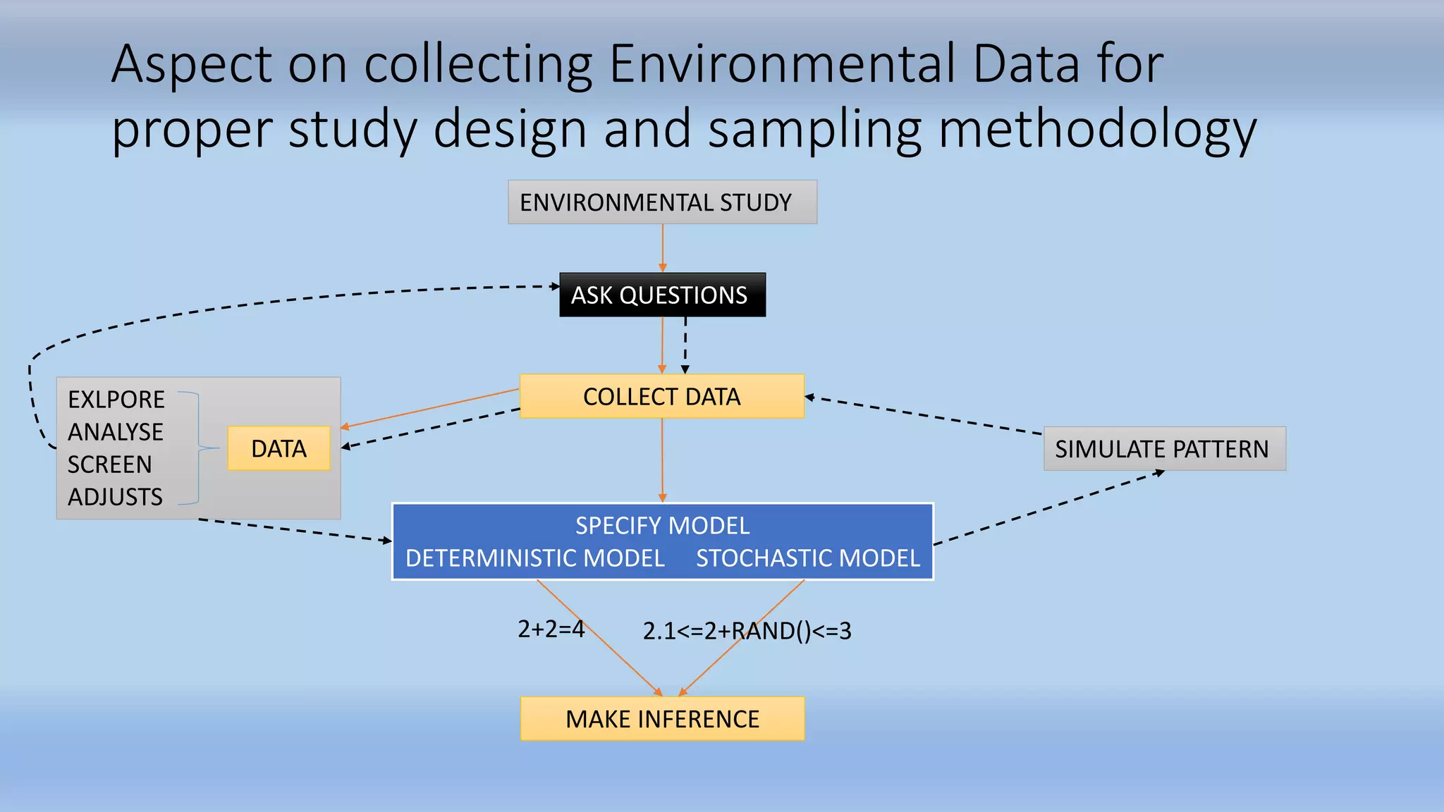
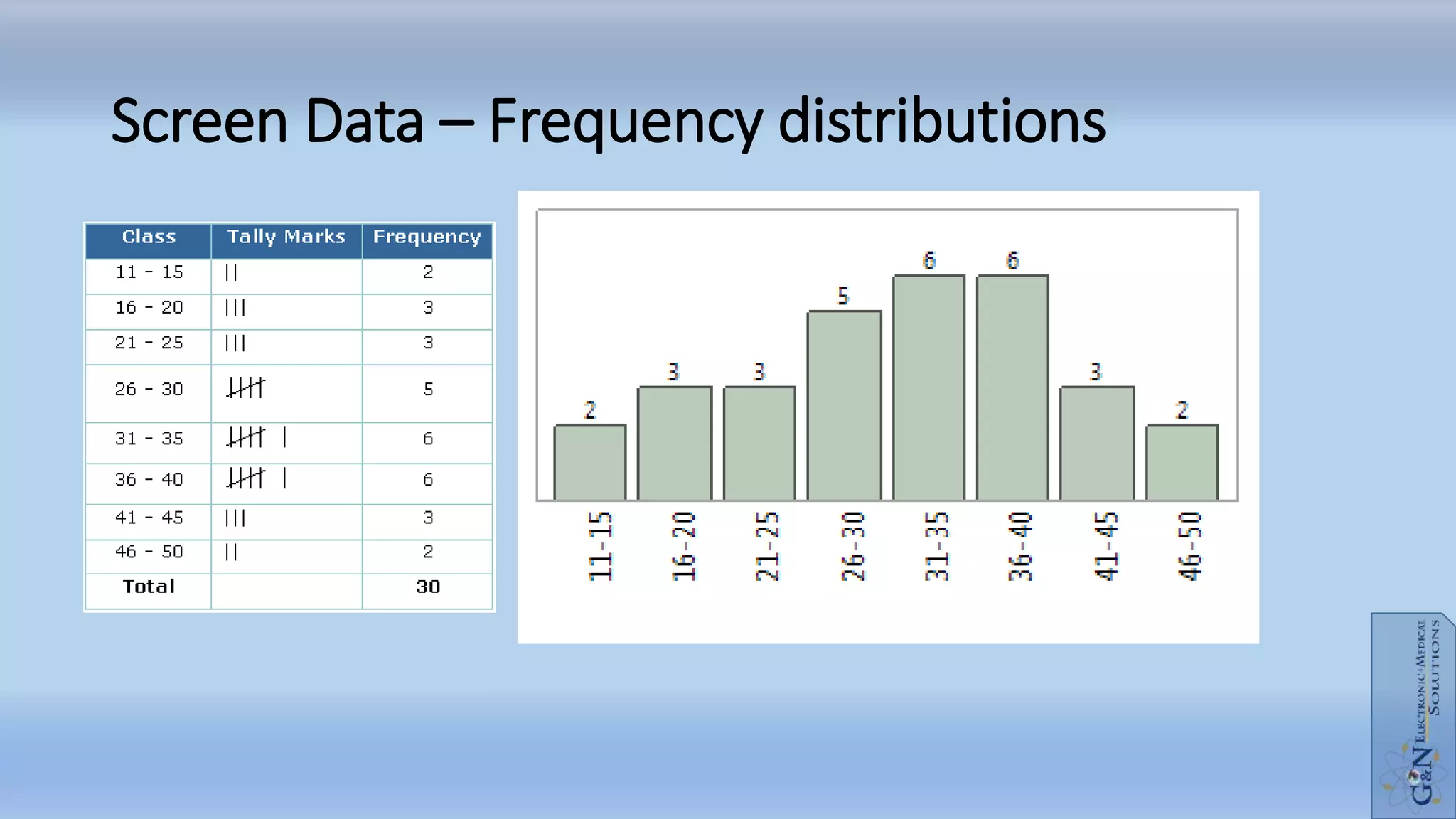
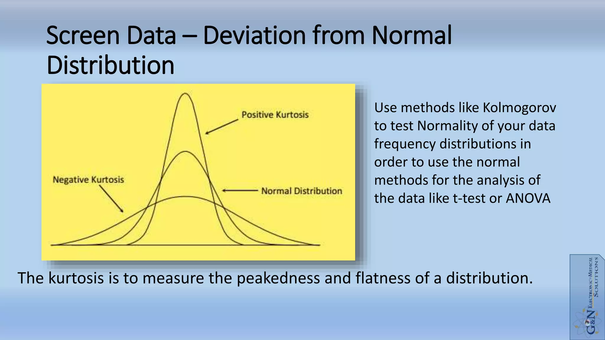
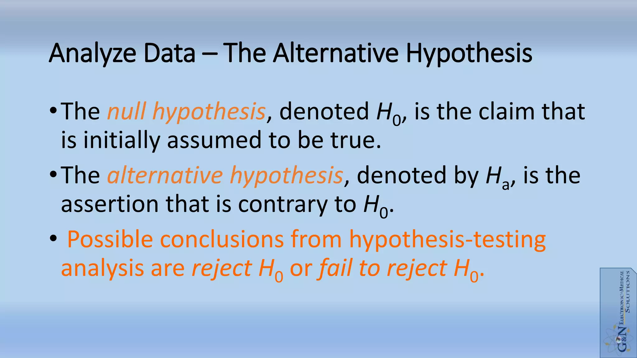
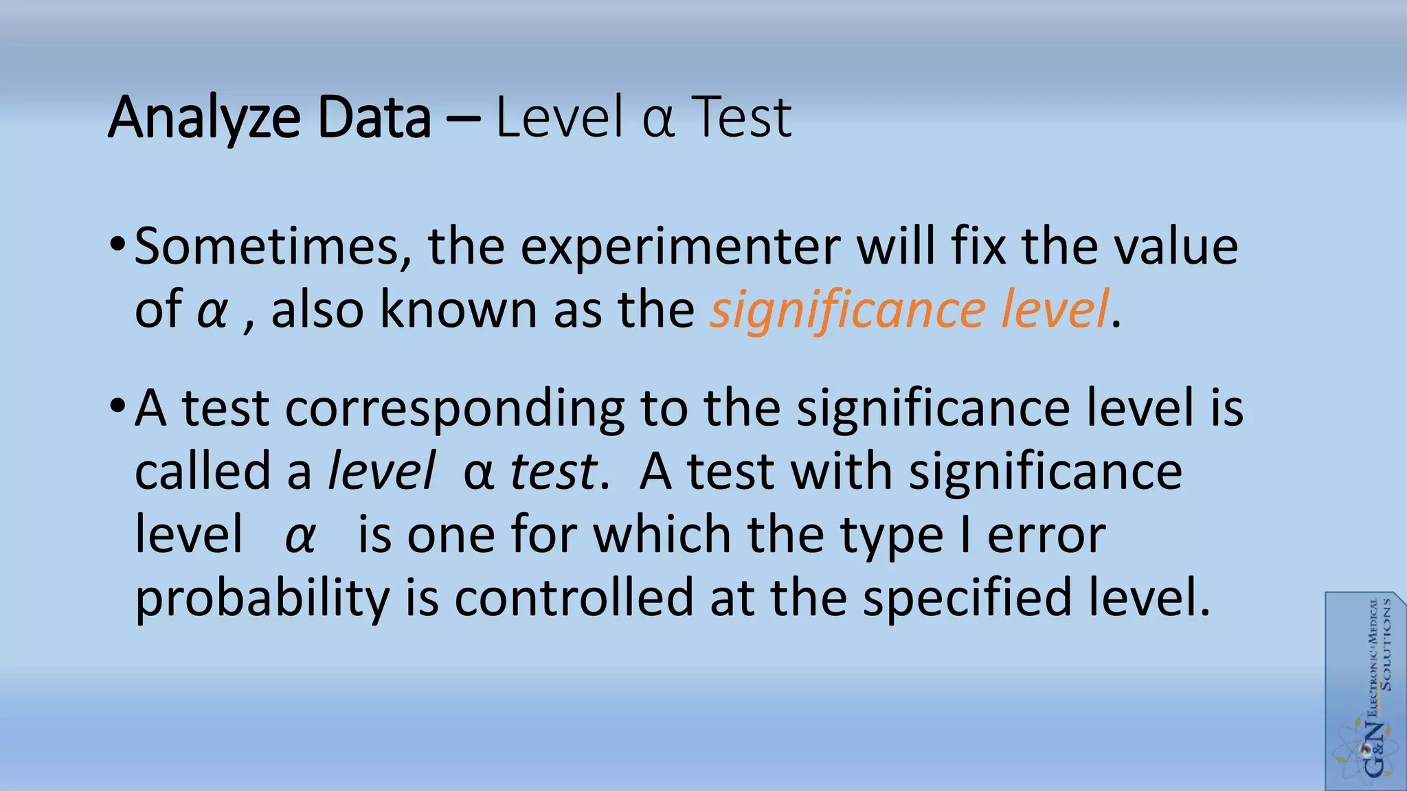
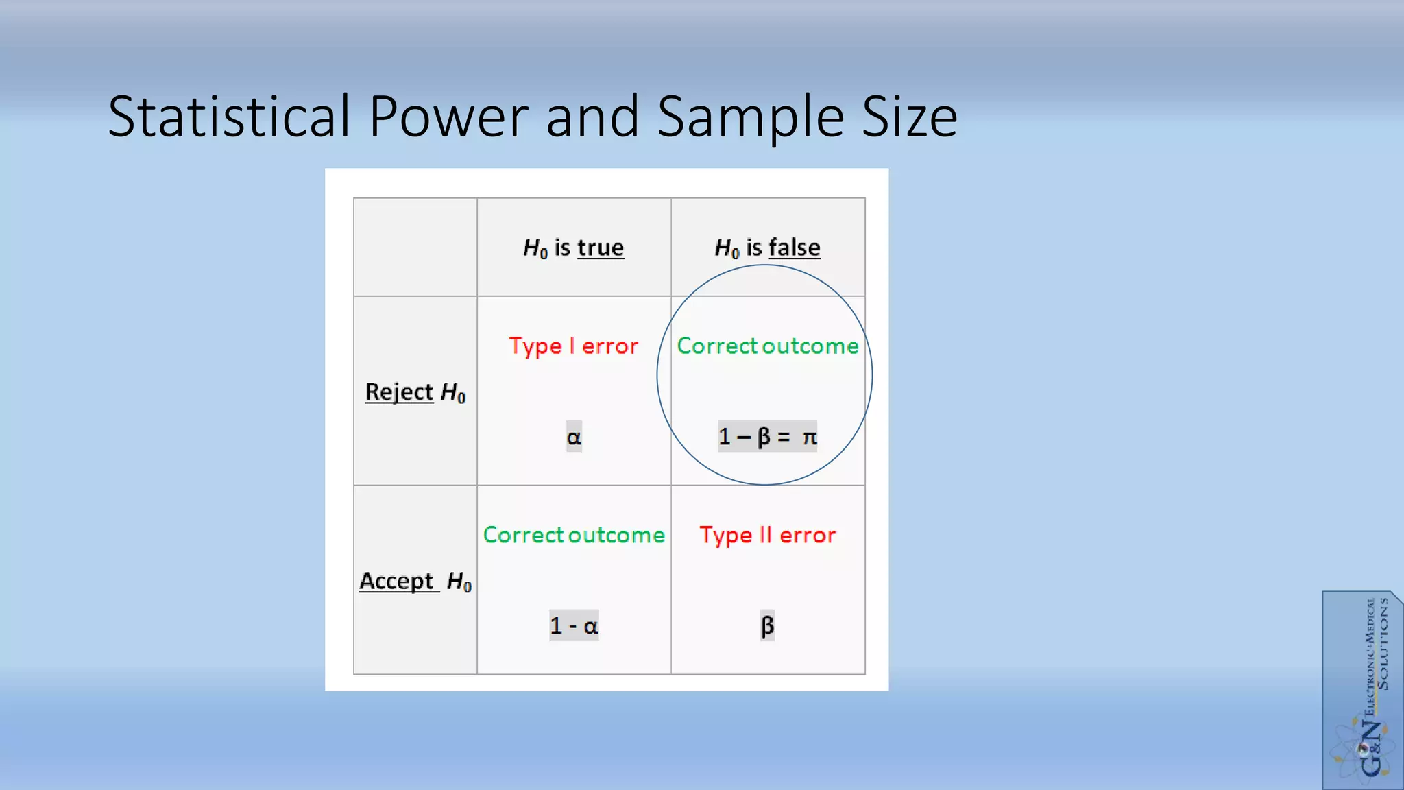
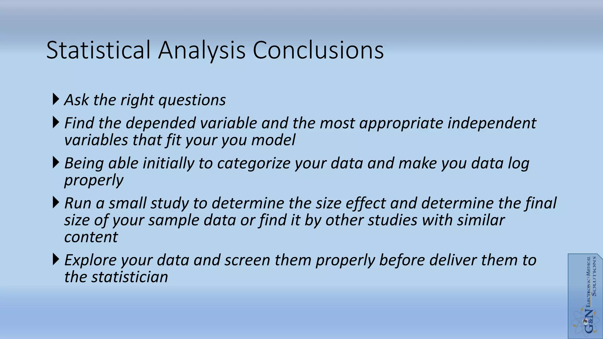
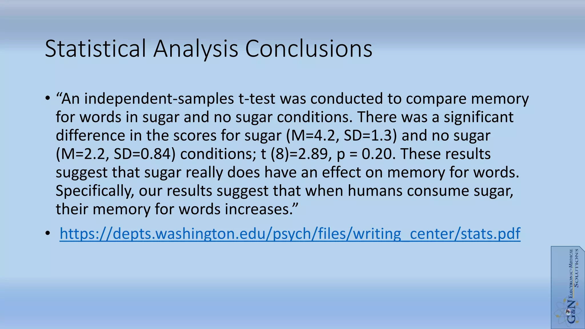
Call Girls in Defence Colony Delhi 💯Call Us 🔝8264348440🔝
Environmental statistics
1. Statistical analysis of data in
environmental studies.
Principles of Analysis
Dr. Georgios A Kounis
SCHOOL OF THE ENVIRONMENT - Department of Environment
9 Jul 2018 to 15 Jul 2018
Skyros
2. Aspect on collecting Environmental Data for
proper study design and sampling methodology
ENVIRONMENTAL STUDY
COLLECT DATA
SPECIFY MODEL
DETERMINISTIC MODEL STOCHASTIC MODEL
EXLPORE
ANALYSE
SCREEN
ADJUSTS
DATA SIMULATE PATTERN
MAKE INFERENCE
ASK QUESTIONS
2+2=4 2.1<=2+RAND()<=3
3. Research question.
• Good research has the characteristic that its purpose is to address a
single clear and explicit research question
• Weakest of all, however, are those studies that have no research
question at all and whose design simply is to collect a wide range of
data and then to ‘trawl’ the data looking for ‘interesting’ or
‘significant’ associations.
• Be knowledgeable about the area you wish to research.
• Widen the base of your experience, explore related areas, and talk to other
researchers and practitioners in the field you are surveying.
• Avoid the pitfalls of: allowing a decision regarding methods to decide the
questions to be asked.
4. Collecting Data Parameters
• In statistics, a population is a set of similar items or events which is of
interest for some question or experiment. A statistical population can
be a group of existing objects (e.g. the set of all stars within the Milky
Way galaxy) or a hypothetical and potentially infinite group of objects
conceived as a generalization from experience (e.g. the set of all
possible hands in a game of poker).
• Importantly, we infer characteristics of the population from the
sample; Thus, the entire realm of inferential statistics applies when
we seek to draw conclusions from a sample about the underlying
population
5. Collecting Data Parameters
• In statistics a data sample is a set of data collected and/or selected
from a statistical population by a defined procedure.The elements of
a sample are known as sample points, sampling units or
observations.
In statistics, a simple random sample is
a subset of individuals where each
individual is chosen randomly and entirely
by chance, such that each individual has
the same probability of being chosen at
any stage during the sampling process.
6. Collecting Data Parameters
• A variable is a property of an object/individual of the sample like hair
color from a sample of humans and all variables/observation in a
study create the Data's
• Data's might be Categorical or Numerical
• Categorical data consist of Discrete Variables usually
• Discrete Variables
• Limited number of values (like gender or YES/NO)Two Categories or binary
or dichotomous variables.
• Color is discrete but has more that two categories and thus called Nominal
• If Nominal Data have ordering property like Low/Medium/High then the data
are called Ordinal
7. Collecting Data Parameters
• Numerical Variables
• Limited Or Unlimited number of values.
• Discrete Numerical Variables when numerical values are limited like
1,2,3,4,5,>5.
• Continues Numerical Variables when they can be whatever form of
measurement like height, width, temperature, counts, proportions, time at
death, time series etc
8. Inferring depended parameters form
independent data (variables)
• In most, but not all, studies, our environmental question requires that
we collect data on two or more variables in which one or more
variables are considered as “independent” variables and one or more
are considered as “dependent” variables.
• Independent variable... is also known as "x ", "predictor“, "regressor,"
"controlled, and/or "input” variable.
• Dependent variable... is also known as "y", "response," "regressand,"
"observed", "outcome“, "experimental“, and/or "output" variable.
9. Explore Data – Mean Values
• The "mean" is the "average" you're used to, where you add up all the
numbers and then divide by the number of numbers.
• The "median" is the "middle" value in the list of numbers. To find the
median, your numbers have to be listed in numerical order from
smallest to largest
• The "mode" is the value that occurs most often. If no number in the
list is repeated, then there is no mode for the list.
10. Explore Data – Variances from Mean Values
• Standard Deviation
• The Standard Deviation is a measure of how spread out numbers are.
• Its symbol is σ (the Greek letter sigma)
• The formula is easy: it is the square root of the Variance. So now you ask,
"What is the Variance?"
• Variance
• The Variance is defined as:
• The average of the squared differences from the Mean.
12. Screen Data – Normal Distribution
The simplest case of a normal distribution is known as the standard normal distribution. This is a special case
when mean value is 0 and standard deviation is 1.
Generally all physical variables which are randomly selected from a population follow a normal distribution
pattern
13. Screen Data – Deviation from Normal
Distribution
In a lot of analyses having a normal distribution is an assumption, but most of them are robust against violations
so the importance doesn't really matter that much as long as you have a decent sample size.
14. Screen Data – Deviation from Normal
Distribution
The kurtosis is to measure the peakedness and flatness of a distribution.
Use methods like Kolmogorov
to test Normality of your data
frequency distributions in
order to use the normal
methods for the analysis of
the data like t-test or ANOVA
15. Adjust Data – Logarithm of the Variable
The figures above illustrate an example of this concept. Figure on the
left shows a set of cycle-time data; Figure on the right shows the same
data transformed with the natural logarithm.
16. Analyze Data – The Alternative Hypothesis
•The null hypothesis, denoted H0, is the claim that
is initially assumed to be true.
•The alternative hypothesis, denoted by Ha, is the
assertion that is contrary to H0.
• Possible conclusions from hypothesis-testing
analysis are reject H0 or fail to reject H0.
17. Analyze Data – The Alternative Hypothesis
•H0 may usually be considered the skeptic’s
hypothesis: Nothing new or interesting
happening here! (And anything “interesting”
observed is due to chance alone.)
•Ha may usually be considered the researcher’s
hypothesis.
18. Analyze Data – The Alternative Hypothesis
•H0 is always stated as an equality claim involving
parameters.
•Ha is an inequality claim that contradicts H0. It
may be one-sided (using either > or <) or two-
sided (using ≠).
19. Analyze Data – Errors in Hypothesis Testing
•A type I error consists of rejecting the null
hypothesis H0 when it was true.
•A type II error consists of not rejecting H0 when
H0 is false.
• α and β are the probabilities of type I and type II
error, respectively.
20. Analyze Data – Level α Test
•Sometimes, the experimenter will fix the value
of α , also known as the significance level.
•A test corresponding to the significance level is
called a level α test. A test with significance
level α is one for which the type I error
probability is controlled at the specified level.
21. Analyze Data – Rejection Region: α and β
•Suppose an experiment and a sample size are
fixed, and a test statistic is chosen. Decreasing
the size of the rejection region to obtain a
smaller value of α results in a larger value of β
for any particular parameter value consistent
with Ha.
22. Analyze Data – P – Value –Typically 0.05 or
0.01
•The P-value is the smallest level of significance at
which H0 would be rejected when a specified
test procedure is used on a given data set.
0
1. -value
reject at a level of
P
H
0
2. -value
do not reject at a level of
P
H
23. Analyze Data – Statistical Versus Practical
Significance
•Be careful in interpreting evidence when the
sample size is large, since any small departure
from H0 will almost surely be detected by a test
(statistical significance), yet such a departure
may have little practical significance.
24. We wish to Reject Null Hypothesis and accept the alternative.
IF the Null Hypothesis is true, how often are we likely to reject it?
As small as possible is acceptable and it is the alpha error and is given by the level of
significance chosen at .05 or .01 : Type I Error False Posetive
IF the Alternative Hypothesis is true , how often do we reject it?
We wish this error also to be as small as possible and is the beta error : Type II Error
False Negative
Power (π) = (1- β) = probability of detecting a difference when a
difference does exist As large as possible
– how sensitive your test is to the existing difference between the
compared samples
Statistical Power and Sample Size.
VERY IMPORTANT
26. • Generally, the minimal sufficient (acceptable) value of power is 0.80
• π ≥ 0.80
How do we know that power is large enough?
27. • 1) Before gathering data
• To determine the minimal sample size needed to have desired power
in statistical testing (to detect a particular effect size)
• 2) After gathering data
• To determine the magnitude of power that your statistical test will
have given the sample parameters (n and s) and the magnitude of the
effect that you want to detect
Analysis of power is performed:
28. Sample size (n)
Standard deviation (s)
Alpha level (α )
Size of effect/difference that you want to detect
Type of statistical test performed
Power depends on:
29. Specify Model.
Type of
Data
Categorical
Type of
Categorization
One Categorical
Variable
Two
Categorical
Variables
Goodness-of-fit 𝜒2
Contingency Tables 𝜒2
Measurement
Type of
Question
Relationships
Number of
Predictors
One
Multiple
Measurements
Continuous
Ranks
Multiple
Regression
Primary Interest
Degree of
Relationship
Form of
Relationship
Pearson
correlation
Regression
Spearman’s rs
Differences
Number
of Groups
Two
Multiple
Relation
Between
Samples
Number
of Groups
Independent
Two-Sample
t-test
Dependent
Independent
Dependent
Mann-
Whitney
Related
sample t-test
Wilcoxon
Repeated
MEasures
Friedman
Number of
indep. Var.
One
Multiple
Factorial
ANOVA
One-way
ANOVA
Kruskal-
Wallis
30. Contingency Tables.
Common Tools
Count
Total %
Col %
Row %
Right Handed Left Handed
Male
43
43,00
49,43
82,69
9
9,00
69,23
17,31
52
52,00
Female
44
44,00
50,57
91,67
4
4,00
30,77
8,33
48
48,00
87
87,00
13
13,00
100
Further suppose that 100 individuals are
randomly sampled from a very large
population as part of a study of sex
differences in handedness. A
contingency table can be created to
display the numbers of individuals who
are male and right handed, male and
left handed, female and right handed
Suppose there are two variables, sex (male or female) and handedness (right or left
handed).
The table allows users to see at a glance
that the proportion of men who are right
handed is about the same as the
proportion of women who are right
handed although the proportions are not
identical.
33. Ask the right questions
Find the depended variable and the most appropriate independent
variables that fit your you model
Being able initially to categorize your data and make you data log
properly
Run a small study to determine the size effect and determine the final
size of your sample data or find it by other studies with similar
content
Explore your data and screen them properly before deliver them to
the statistician
Statistical Analysis Conclusions
34. Change the data or adjust them to follow normal distributions if they
don’t.
Being able to explain thoroughly the model you wish to follow.
Apply the model and see how the simulation patterns work if it is an
arithmetic model.
Finally being able to write properly the results in the correct
statistical way according to your results.
Statistical Analysis Conclusions
36. • “An independent-samples t-test was conducted to compare memory
for words in sugar and no sugar conditions. There was a significant
difference in the scores for sugar (M=4.2, SD=1.3) and no sugar
(M=2.2, SD=0.84) conditions; t (8)=2.89, p = 0.20. These results
suggest that sugar really does have an effect on memory for words.
Specifically, our results suggest that when humans consume sugar,
their memory for words increases.”
• https://depts.washington.edu/psych/files/writing_center/stats.pdf
Statistical Analysis Conclusions
Editor's Notes
Δημιουργία περιοχών ενδιαφέροντος. Ζώνες συναγερμού και προσυναγερμού.
Οθόνες ενδείξεων εισερχόμενων σημάτων και καμπύλες παρακολούθησης στόχων
Δημιουργία περιοχών ενδιαφέροντος. Ζώνες συναγερμού και προσυναγερμού.
Οθόνες ενδείξεων εισερχόμενων σημάτων και καμπύλες παρακολούθησης στόχων
Δημιουργία περιοχών ενδιαφέροντος. Ζώνες συναγερμού και προσυναγερμού.
Οθόνες ενδείξεων εισερχόμενων σημάτων και καμπύλες παρακολούθησης στόχων
Δημιουργία περιοχών ενδιαφέροντος. Ζώνες συναγερμού και προσυναγερμού.
Οθόνες ενδείξεων εισερχόμενων σημάτων και καμπύλες παρακολούθησης στόχων
Δημιουργία περιοχών ενδιαφέροντος. Ζώνες συναγερμού και προσυναγερμού.
Οθόνες ενδείξεων εισερχόμενων σημάτων και καμπύλες παρακολούθησης στόχων
Δημιουργία περιοχών ενδιαφέροντος. Ζώνες συναγερμού και προσυναγερμού.
Οθόνες ενδείξεων εισερχόμενων σημάτων και καμπύλες παρακολούθησης στόχων