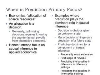
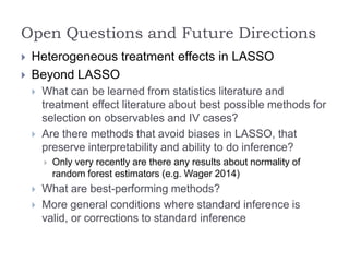
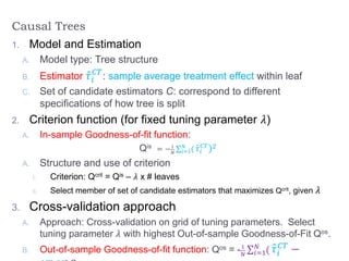
This document summarizes a discussion between Susan Athey and Guido Imbens on the relationship between machine learning and causal inference. It notes that while machine learning excels at prediction problems using large datasets, it has weaknesses when it comes to causal questions. Econometrics and statistics literature focuses more on formal theories of causality. The document proposes combining the strengths of both fields by developing machine learning methods that can estimate causal effects, accounting for issues like endogeneity and treatment effect heterogeneity. It outlines some open problems and directions for future research at the intersection of these fields.


![Using ML for the first stage of IV
IV assumptions
𝑌𝑖(𝑤) ⊥ 𝑍𝑖|𝑋𝑖
See Imbens and Rubin (2015) for extensive review
First stage estimation: instrument selection and
functional form
𝐸[𝑊𝑖|𝑍𝑖, 𝑋𝑖] This is a prediction problem where
interpretability is less important
Variety of methods available
Belloni, Chernozhukov, and Hansen (2010); Belloni,
Chen, Chernozhukov and Hansen (2012) proposed
LASSO
Under some conditions, second stage inference occurs as usual
Key: second-stage is immune to misspecification in the first
stage](https://image.slidesharecdn.com/nbercausalpredictionv111-150817123705-lva1-app6891/85/Machine-Learning-and-Causal-Inference-15-320.jpg)

![Using Trees to Estimate Causal Effects
Model:
𝑌𝑖 = 𝑌𝑖 𝑊𝑖 =
𝑌𝑖(1) 𝑖𝑓 𝑊𝑖 = 1,
𝑌𝑖(0) 𝑜𝑡ℎ𝑒𝑟𝑤𝑖𝑠𝑒.
Suppose random assignment of Wi
Want to predict individual i’s treatment effect
𝜏𝑖 = 𝑌𝑖 1 − 𝑌𝑖(0)
This is not observed for any individual
Not clear how to apply standard machine learning tools
Let
𝜇(𝑤, 𝑥) = 𝔼[𝑌𝑖|𝑊𝑖 = 𝑤, 𝑋𝑖 = 𝑥]
𝜏(𝑥) = 𝜇(1, 𝑥) − 𝜇(0, 𝑥)](https://image.slidesharecdn.com/nbercausalpredictionv111-150817123705-lva1-app6891/85/Machine-Learning-and-Causal-Inference-23-320.jpg)
![Using Trees to Estimate Causal Effects
𝜇(𝑤, 𝑥) = 𝔼[𝑌𝑖|𝑊𝑖 = 𝑤, 𝑋𝑖 = 𝑥]
𝜏(𝑥) = 𝜇(1, 𝑥) − 𝜇(0, 𝑥)
Approach 1: Analyze two groups
separately
Estimate 𝜇(1, 𝑥) using dataset where 𝑊𝑖 =
1
Estimate 𝜇(0, 𝑥) using dataset where 𝑊𝑖 =
0
Use propensity score weighting (PSW) if
needed
Do within-group cross-validation to choose
tuning parameters
Construct prediction using
𝜇(1, 𝑥) − 𝜇(0, 𝑥)
Approach 2: Estimate 𝜇(𝑤, 𝑥) using tree
including both covariates
Include PS as attribute if needed
Choose tuning parameters as usual
Construct prediction using
𝜇(1, 𝑥) − 𝜇(0, 𝑥)
Observations
Estimation and cross-validation
not optimized for goal
Lots of segments in Approach
1: combining two distinct ways
to partition the data
Problems with these
approaches
1. Approaches not tailored to the goal
of estimating treatment effects
2. How do you evaluate goodness of
fit for tree splitting and cross-
validation?
𝜏𝑖 = 𝑌𝑖 1 − 𝑌𝑖 0 is not observed
and thus you don’t have ground truth](https://image.slidesharecdn.com/nbercausalpredictionv111-150817123705-lva1-app6891/85/Machine-Learning-and-Causal-Inference-24-320.jpg)
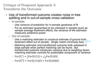
![Proposed Approach 3: Transform the Outcome
Suppose we have 50-50 randomization of
treatment/control
Let 𝑌𝑖
∗
=
2𝑌𝑖 𝑖𝑓 𝑊𝑖 = 1
−2𝑌𝑖 𝑖𝑓 𝑊𝑖 = 0
Then 𝐸 𝑌𝑖
∗
= 2 ⋅ 1
2
𝐸 𝑌𝑖 1 − 1
2
𝐸 𝑌𝑖 0 = 𝐸[𝜏𝑖]
Suppose treatment with probability pi
Let 𝑌𝑖
∗
=
𝑊 𝑖−𝑝
𝑝(1−𝑝)
𝑌𝑖 =
1
𝑝
𝑌 𝑖 𝑖𝑓 𝑊𝑖 = 1
− 1
1−𝑝
𝑌𝑖 𝑖𝑓 𝑊𝑖 = 0
Then 𝐸 𝑌𝑖
∗
= 𝑝1
𝑝
𝐸 𝑌𝑖 1 − (1 − 𝑝) 1
1−𝑝
𝐸 𝑌𝑖 0 = 𝐸[𝜏𝑖]
Selection on observables or stratified experiment
Let 𝑌𝑖
∗
=
𝑊 𝑖−𝑝 𝑋 𝑖
𝑝(𝑋 𝑖)(1−𝑝(𝑋 𝑖))
𝑌𝑖
Estimate 𝑝 𝑥 using traditional methods](https://image.slidesharecdn.com/nbercausalpredictionv111-150817123705-lva1-app6891/85/Machine-Learning-and-Causal-Inference-25-320.jpg)
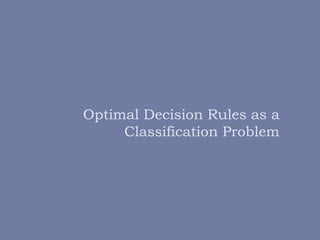
![Model
Outcome Yi incorporates
both costs and benefits
If cost is known, e.g. a
mailing, define outcome to
include cost
Treatment Wi is multi-valued
Attributes Xi observed
Maintain selection on
observables assumption:
𝑌𝑖(𝑤) ⊥ 𝑊𝑖|𝑋𝑖
Propensity score:
Pr 𝑊𝑖 = 𝑤𝑖|𝑋𝑖 = 𝑥𝑖 = 𝑝 𝑤(𝑥)
Optimal policy:
p*(x) = argmaxwE[Yi(w)|Xi=x]
Examples/interpretation
Marketing/web site design
Outcome is voting, purchase,
a click, etc.
Treatment is the offer
Past user behavior used to
define attributes
Selection on observables
justified by past
experimentation (or real-time
experimentation)
Personalized medicine
Treatment plan as a function
of individual characteristics](https://image.slidesharecdn.com/nbercausalpredictionv111-150817123705-lva1-app6891/85/Machine-Learning-and-Causal-Inference-44-320.jpg)
![Learning Policy Functions
ML Literature:
Contextual bandits (e.g., John
Langford), associative
reinforcement learning,
associative bandits, learning
with partial feedback, bandits
with side information, partial
label problem
Cost-sensitive classification
Classifiers (e.g. logit, CART,
SVM) = discrete choice models
Weight observations by
observation-specific weight
Objective function: minimize
classification error
The policy problem
Minimize regret from
suboptimal policy (“policy
regret”)
For 2-choice case:
Procedure with transformed outcome:
Train classifier as if obs. treatment is
optimal:
(features, choice, weight)= (Xi, Wi, 𝑌 𝑖
𝑝(𝑥)
).
Estimated classifier is a possible policy
Result:
The loss from the cost-weighted classifier
(misclassification error minimization)
is the same in expectation
as the policy regret
Intuition
The expected value of the weights
conditional on xi,wi is E[Yi(wi)|Xi=xi]
Implication
Use off-the-shelf classifier to learn
optimal policies, e.g. logit, CART, SVM
Literature considers extensions to multi-
valued treatments (tree of binary](https://image.slidesharecdn.com/nbercausalpredictionv111-150817123705-lva1-app6891/85/Machine-Learning-and-Causal-Inference-45-320.jpg)
![Weighted Classification Trees:
Transformed Outcome Approach
Interpretation
This is analog of using the transformed outcome approach for
heterogeneous treatment effects, but for learning optimal policies
The in-sample and out-of-sample criteria have high variance, and don’t
adjust for actual sample proportions or predictable variation in outcomes
as function of X
Comparing two policies: Loss A – Loss B with NT units
Policy A & B
Rec’s
Treated
Units
Control
Units
Expected value of sum
Region S10
A: Treat
B: No Treat
−
1
𝑁 𝑇
𝑌 𝑖
𝑝
1
𝑁 𝑇
𝑌 𝑖
1−𝑝
−Pr(𝑋𝑖 ∈ 𝑆10)𝐸[𝜏𝑖|𝑋𝑖 ∈ 𝑆10]
Region S01
A: No Treat
B: Treat
1
𝑁 𝑇
𝑌 𝑖
𝑝
−
1
𝑁 𝑇
𝑌 𝑖
1−𝑝
Pr(𝑋𝑖 ∈ 𝑆01)𝐸[𝜏𝑖|𝑋𝑖 ∈ 𝑆01]](https://image.slidesharecdn.com/nbercausalpredictionv111-150817123705-lva1-app6891/85/Machine-Learning-and-Causal-Inference-46-320.jpg)
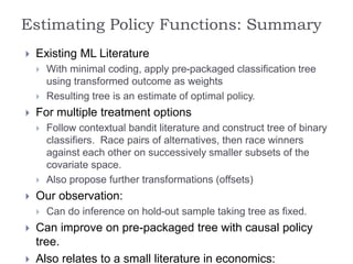
![Alternative: Causal Policy Tree
(Athey-Imbens 2015-WIP)
Improve by same logic that causal trees improved on transformed
outcome
In sample
Estimate treatment effect 𝜏(𝑥)within leaves using actual proportion treated
in leaves (average treated outcomes – average control outcomes)
Split based on classification costs, using sample average treatment effect
to estimate cost within a leaf. Equivalent to modifying TO to adjust for
correct leaf treatment proportions.
Comparing two policies: Loss A – Loss B with NT
units
Policy A & B
Rec’s
Treated
Units
Control
Units
Expected value of sum
Region S10
A: Treat
B: No Treat
−
1
𝑁 𝑇 𝜏(𝑆10) −
1
𝑁 𝑇
𝜏(𝑆10) −Pr(𝑋𝑖 ∈ 𝑆10)𝐸[𝜏𝑖|𝑋𝑖 ∈ 𝑆10]
Region S01
A: No Treat
B: Treat
1
𝑁 𝑇 𝜏(𝑆01)
1
𝑁 𝑇
𝜏(𝑆10) Pr(𝑋𝑖 ∈ 𝑆01)𝐸[𝜏𝑖|𝑋𝑖 ∈ 𝑆01]](https://image.slidesharecdn.com/nbercausalpredictionv111-150817123705-lva1-app6891/85/Machine-Learning-and-Causal-Inference-47-320.jpg)
![Alternative: Causal Policy Tree
(Athey-Imbens 2015-WIP)
Comparing two policies: Loss A – Loss B with NT
units
Policy A & B
Rec’s
Treated
Units
Control
Units
Expected value of sum
Region S10
A: Treat
B: No Treat
−
1
𝑁 𝑇
𝜏(𝑆10) −
1
𝑁 𝑇
𝜏(𝑆10) −Pr(𝑋𝑖 ∈ 𝑆10)𝐸[𝜏𝑖|𝑋𝑖 ∈ 𝑆10]
Region S01
A: No Treat
B: Treat
1
𝑁 𝑇 𝜏(𝑆01)
1
𝑁 𝑇 𝜏(𝑆01)
Pr(𝑋𝑖 ∈ 𝑆01)𝐸[𝜏𝑖|𝑋𝑖 ∈ 𝑆01]
Policy A & B
Rec’s
Treated
Units
Control
Units
Expected value of sum
Region S10
A: Treat
B: No Treat
−
1
𝑁 𝑇
𝑌 𝑖
𝑝
1
𝑁 𝑇
𝑌 𝑖
1−𝑝
−Pr(𝑋𝑖 ∈ 𝑆10)𝐸[𝜏𝑖|𝑋𝑖 ∈ 𝑆10]
Region S01
A: No Treat
B: Treat
1
𝑁 𝑇
𝑌 𝑖
𝑝 −
1
𝑁 𝑇
𝑌 𝑖
1−𝑝
Pr(𝑋𝑖 ∈ 𝑆01)𝐸[𝜏𝑖|𝑋𝑖 ∈ 𝑆01]](https://image.slidesharecdn.com/nbercausalpredictionv111-150817123705-lva1-app6891/85/Machine-Learning-and-Causal-Inference-48-320.jpg)