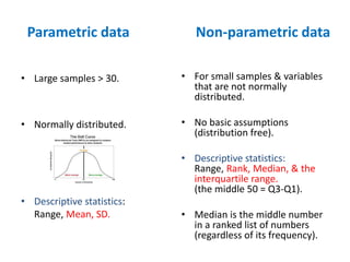
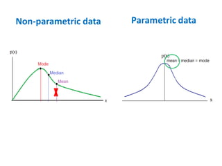
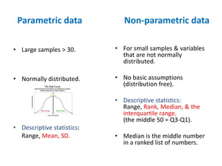
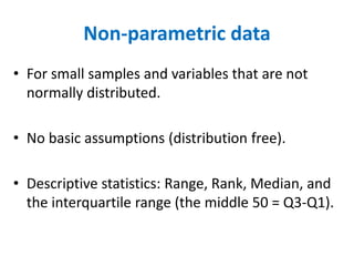
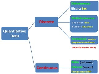
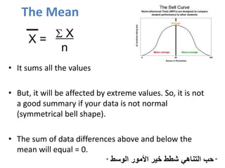
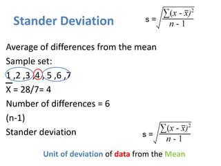
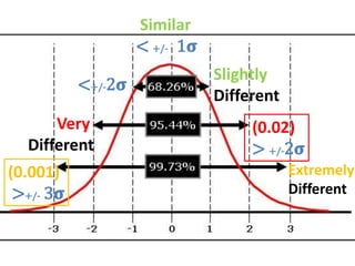
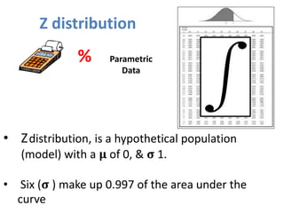
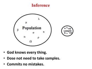
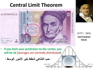
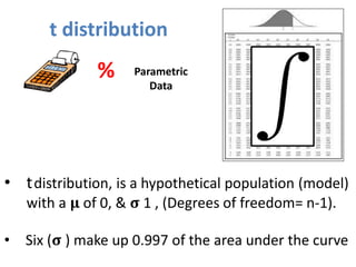
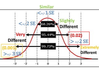
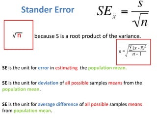
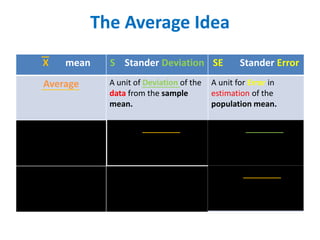
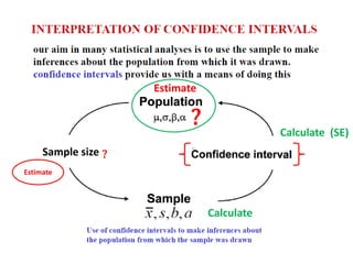
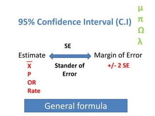
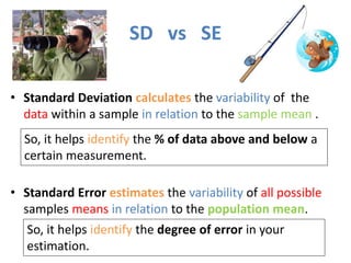
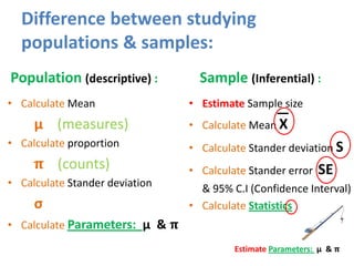
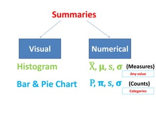
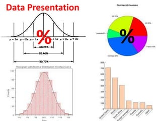
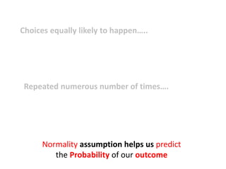
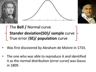
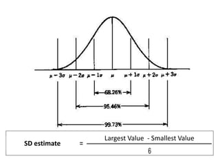
- The document discusses parametric and non-parametric data, describing key differences. Non-parametric data is for small samples and variables that are not normally distributed, requiring no assumptions. Descriptive statistics include range, rank, median, and interquartile range. - It also covers topics like mean, standard deviation, standard error, confidence intervals, and the normal and t-distributions as they relate to parametric statistical analysis of sample and population data. The central limit theorem is also referenced.

1. Basics in Epidemiology & Biostatistics
Hashem Alhashemi MD, MPH, FRCPC
Assistant Professor, KSAU-HS

2. • Large samples > 30.
• Normally distributed.
• Descriptive statistics:
Range, Mean, SD.
Non-parametric data
• For small samples & variables
that are not normally
distributed.
• No basic assumptions
(distribution free).
• Descriptive statistics:
Range, Rank, Median, & the
interquartile range.
(the middle 50 = Q3-Q1).
• Median is the middle number
in a ranked list of numbers
(regardless of its frequency).
Parametric data

3. Non-parametric data

4. The Mean
• It sums all the values (great digital summary ).
• But, it will be affected by extreme values. So, it is not
a good summary if your data is not normal
(symmetrical bell shape).
• The sum of data differences above and below the
mean will equal = 0.
"‫الوسط‬ ‫األمور‬ ‫خير‬ ‫شطط‬ ‫التناهي‬ ‫حب‬"

5. Stander Deviation
Average of differences from the mean (Squared-SS)
Sample set:
1 ,2 ,3 ,4 , 5 ,6 ,7
X = 28/7= 4
Number of differences = 6
(n-1)
Stander deviation
Unit of deviation of data from the Mean

6. Differences?

7. Similar
< +/- 1𝛔
Slightly
Different
Very
Different
Extremely
Different
(0.02)
> +/-2𝛔
(0.001)
>+/- 3𝛔
<+/-2𝛔

8. • Zdistribution, is a hypothetical population
(model) with a 𝛍 of 0, & 𝛔 1.
• Six (𝛔 ) make up 0.997 of the area under the
curve
Z distribution
Parametric
Data
Population
%

9. • God knows every thing.
• Dose not need to take samples.
• Commits no mistakes.

10. Central Limit Theorem
• The mean of all possible sample means will be
approximately equal to the mean of the
population.
• The distribution of all possible sample means
will be normal.
• If you limit your prediction to the center, you
will be ok (averages are normally distributed)
(1777 – 1855)
"‫الوسط‬ ‫األمور‬ ‫خير‬ ‫شطط‬ ‫التناهي‬ ‫حب‬"
Carl Friedrich
Gauss

11. • tdistribution, is a hypothetical population (model)
with a 𝛍 of 0, & 𝛔 1 , (Degrees of freedom= n-1).
• Six (𝛔 ) make up 0.997 of the area under the curve
t distribution
Parametric
Data
Sample
Sampling distribution
%

12. Similar
<+/-1 SE
Slightly
Different
Very
Different
Extremely
Different
(0.02)
> +/-2 SE
(0.001)
>+/- 3 SE
<+/-2 SE

13. Stander Error
SE is the unit for error in estimating the population mean.
SE is the unit for deviation of all possible samples means from the
population mean.
SE is the unit for average difference of all possible samples means
from population mean.
n because S is a root product of the variance.

14. The Average Idea
SE Stander ErrorS Stander DeviationX mean
A unit for Error in
estimation of the
population mean.
A unit of Deviation of the
data from the sample
mean.
Average
A unit for Deviation of
all possible samples
means from the
population mean.
A unit for Average of
differences of the data
from the sample mean.
A unit for Average of
differences of all
possible samples means
from population mean.

15. A Fancy World made of
%s & Averages
Biostatistics

16. Sample size
Estimate
Calculate
Calculate (SE)
?
?
Estimate

17. 95% Confidence Interval (C.I)
SE
Stander of
Error
+/- 2 SE
μ
π
Ω
λ
Estimate Margin of Error
X
P
OR
Rate
General formula

18. SD vs SE
• Standard Deviation calculates the variability of the
data within a sample in relation to the sample mean .
• Standard Error estimates the variability of all possible
samples means in relation to the population mean.
So, it helps identify the % of data above and below a
certain measurement.
So, it helps identify the degree of error in your
estimation.

19. A Fancy World made of
Biostatistics
Averages & %s

20. Population (descriptive) :
• Calculate Mean
μ (measures)
• Calculate proportion
𝛑 (counts)
• Calculate Stander deviation
σ
• Calculate Parameters: μ & 𝛑
Sample (Inferential) :
• Estimate Sample size
• Calculate Mean X
• Calculate Stander deviation S
• Calculate Stander error SE
& 95% C.I (Confidence Interval)
• Calculate Statistics
Difference between studying
populations & samples:
Estimate Parameters: μ & 𝛑

21. END

22. • Large samples > 30.
• Normally distributed.
• Descriptive statistics:
Range, Mean, SD.
Non-parametric data
• For small samples & variables
that are not normally
distributed.
• No basic assumptions
(distribution free).
• Descriptive statistics:
Range, Rank, Median, & the
interquartile range.
(the middle 50 = Q3-Q1).
• Median is the middle number
in a ranked list of numbers.
Parametric data

23. Non-parametric data
• For small samples and variables that are not
normally distributed.
• No basic assumptions (distribution free).
• Descriptive statistics: Range, Rank, Median, and
the interquartile range (the middle 50 = Q3-Q1).

24. Count
Quantitative
Data
Discrete
Continuous
Binomial (Binary) :
Sex
Ratio (real zero) /
Interval (no zero)
Temperature/BP
Multinomial :
1-Categorical : Race
2-Ordinal: Education
3-Numerical: number
pregnancies/residents
Measure

25. Non-parametric data
• For small samples and variables that are not
normally distributed.
• No basic assumptions (distribution free).
• Descriptive statistics: Range, Rank, Median, and
the interquartile range (the middle 50 = Q3-Q1).

26. Differences?

27. Objectives
• Definitions.
• Types of Data.
• Data summaries.
• Mean Χ , Stander deviation S.
• Stander Error SE, Confidence interval C.I of μ .

28. Quantitative
Data
Discrete
Continuous
Dichotomous:
Binary: Sex
Multichotomous:
1-No order : Race
2-Ordinal: Education
Numerical: number
pregnancies/residents
Ratio (real zero) /
Interval (no zero)
Temperature/BP
(Non-Parametric Data)

29. Quantitative
Data
Discrete
Continuous
Categorical :
1- Di-chotomous:
Sex
2- Multi-chotomous:
Race,Education
Numerical:
number of
pregnancies/residents
Ratio (real zero) /
Interval (no zero)
Temperature/BP
Types of
Data Count
Non-Parametric Data
Parametric Data
Parametric Data

30. Summaries
Visual Numerical
X, 𝛍, s, 𝛔Histogram
P, 𝛑, s, 𝛔Bar & Pie Chart (Counts)
Categories
(Measures)
Any value

31. Data Presentation
%%

32. Normality & Approximation to Normality
Why?

33. Approximation to Normality
• If choices are equally likely to happen
• If repeated numerous number of times
• It will look normal.
• Whether it was a coin or a dice
(Di-chotomous or Multi-chotomous)

34. Normality & Approximation to Normality
Clinical Relevance?

35. Choices equally likely to happen…..
i.e. Out come of interest probability is unknown
(Research ethics)
Repeated numerous number of times….
i.e. Large sample size
Normality assumption helps us predict
the Probability of our outcome

36. The Bell / Normal curve
Stander deviation(SD)/ sample curve
True error (SE)/ population curve
• Was first discovered by Abraham de Moivre in 1733.
• The one who was able to reproduce it and identified
it as the normal distribution (error curve) was Gauss
in 1809.

37. De Moivre had hoped for a chair of
mathematics, but foreigners were at a
disadvantage, so although he was free
from religious discrimination, he still
suffered discrimination as a Frenchman in
England.
Born 1667 in Champagne, France
Died 1754 in London, England

38. Largest Value - Smallest Value
SD estimate