Downloaded 198 times


![Likelihood-free Methods
Introduction
Monte Carlo basics
Monte Carlo basics
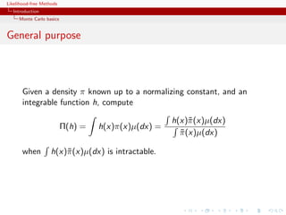
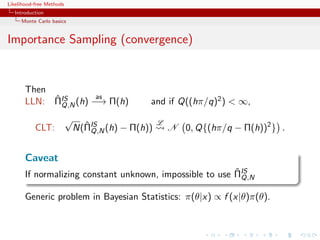
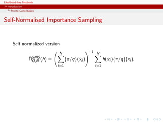
Generate an iid sample x1 , . . . , xN from π and estimate Π(h) by
N
ΠMC (h) = N −1
ˆ
N h(xi ).
i=1
ˆ as
LLN: ΠMC (h) −→ Π(h)
N
If Π(h2 ) = h2 (x)π(x)µ(dx) < ∞,
√ L
CLT: ˆ
N ΠMC (h) − Π(h)
N N 0, Π [h − Π(h)]2 .](https://image.slidesharecdn.com/romabc-120120013357-phpapp02/85/ABC-in-Roma-5-320.jpg)
![Likelihood-free Methods
Introduction
Monte Carlo basics
Monte Carlo basics
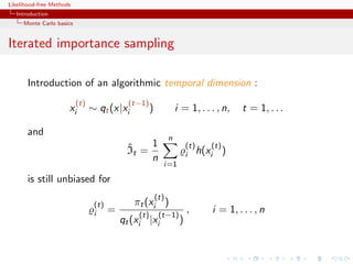
Generate an iid sample x1 , . . . , xN from π and estimate Π(h) by
N
ΠMC (h) = N −1
ˆ
N h(xi ).
i=1
ˆ as
LLN: ΠMC (h) −→ Π(h)
N
If Π(h2 ) = h2 (x)π(x)µ(dx) < ∞,
√ L
CLT: ˆ
N ΠMC (h) − Π(h)
N N 0, Π [h − Π(h)]2 .
Caveat
Often impossible or inefficient to simulate directly from Π](https://image.slidesharecdn.com/romabc-120120013357-phpapp02/85/ABC-in-Roma-6-320.jpg)


![Likelihood-free Methods
Introduction
Population Monte Carlo
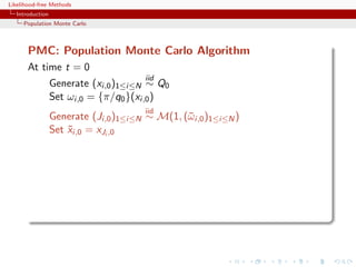
PMC: Population Monte Carlo Algorithm
At time t = 0
iid
Generate (xi,0 )1≤i≤N ∼ Q0
Set ωi,0 = {π/q0 }(xi,0 )
iid
Generate (Ji,0 )1≤i≤N ∼ M(1, (¯ i,0 )1≤i≤N )
ω
Set xi,0 = xJi ,0
˜
At time t (t = 1, . . . , T ),
ind
Generate xi,t ∼ Qi,t (˜i,t−1 , ·)
x
Set ωi,t = {π(xi,t )/qi,t (˜i,t−1 , xi,t )}
x
iid
Generate (Ji,t )1≤i≤N ∼ M(1, (¯ i,t )1≤i≤N )
ω
Set xi,t = xJi,t ,t .
˜
[Capp´, Douc, Guillin, Marin, & CPR, 2009, Stat.& Comput.]
e](https://image.slidesharecdn.com/romabc-120120013357-phpapp02/85/ABC-in-Roma-16-320.jpg)


![Likelihood-free Methods
Introduction
Population Monte Carlo
Improving quality
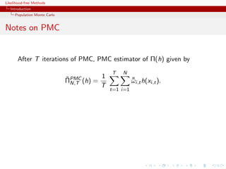
The efficiency of the SNIS approximation depends on the choice of
Q, ranging from optimal
q(x) ∝ |h(x) − Π(h)|π(x)
to useless
ˆ
var ΠSNIS (h) = +∞
Q,N
Example (PMC=adaptive importance sampling)
Population Monte Carlo is producing a sequence of proposals Qt
aiming at improving efficiency
ˆ ˆ
Kull(π, qt ) ≤ Kull(π, qt−1 ) or var ΠSNIS (h) ≤ var ΠSNIS ,∞ (h)
Qt ,∞ Qt−1
[Capp´, Douc, Guillin, Marin, Robert, 04, 07a, 07b, 08]
e](https://image.slidesharecdn.com/romabc-120120013357-phpapp02/85/ABC-in-Roma-20-320.jpg)


![Likelihood-free Methods
Introduction
AMIS
Mixture representation
Deterministic mixture correction of the weights proposed by Owen
and Zhou (JASA, 2000)
The corresponding estimator is still unbiased [if not
self-normalised]
All particles are on the same weighting scale rather than their
own
Large variance proposals Qt do not take over
Variance reduction thanks to weight stabilization & recycling
[K.o.] removes the randomness in the component choice
[=Rao-Blackwellisation]](https://image.slidesharecdn.com/romabc-120120013357-phpapp02/85/ABC-in-Roma-23-320.jpg)


![Likelihood-free Methods
The Metropolis-Hastings Algorithm
Monte Carlo Methods based on Markov Chains
Running Monte Carlo via Markov Chains
Epiphany! It is not necessary to use a sample from the distribution
f to approximate the integral
I= h(x)f (x)dx ,
Principle: Obtain X1 , . . . , Xn ∼ f (approx) without directly
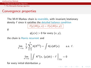
simulating from f , using an ergodic Markov chain with stationary
distribution f
[Metropolis et al., 1953]](https://image.slidesharecdn.com/romabc-120120013357-phpapp02/85/ABC-in-Roma-30-320.jpg)


![Likelihood-free Methods
The Metropolis-Hastings Algorithm
The random walk Metropolis-Hastings algorithm
Acceptance rate
A high acceptance rate is not indication of efficiency since the
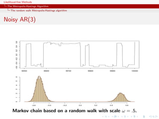
random walk may be moving “too slowly” on the target surface
If average acceptance rate low, the proposed values f (yt ) tend to
be small wrt f (x (t) ), i.e. the random walk [not the algorithm!]
moves quickly on the target surface often reaching its boundaries](https://image.slidesharecdn.com/romabc-120120013357-phpapp02/85/ABC-in-Roma-44-320.jpg)
![Likelihood-free Methods
The Metropolis-Hastings Algorithm
The random walk Metropolis-Hastings algorithm
Rule of thumb
In small dimensions, aim at an average acceptance rate of 50%. In
large dimensions, at an average acceptance rate of 25%.
[Gelman,Gilks and Roberts, 1995]](https://image.slidesharecdn.com/romabc-120120013357-phpapp02/85/ABC-in-Roma-45-320.jpg)


![Likelihood-free Methods
simulation-based methods in Econometrics
Meanwhile, in a Gaulish village...
Similar exploration of simulation-based techniques in Econometrics
Simulated method of moments
Method of simulated moments
Simulated pseudo-maximum-likelihood
Indirect inference
[Gouri´roux & Monfort, 1996]
e](https://image.slidesharecdn.com/romabc-120120013357-phpapp02/85/ABC-in-Roma-49-320.jpg)


![Likelihood-free Methods
simulation-based methods in Econometrics
Method of simulated moments
Given a statistic vector K (y ) with
Eθ [K (Yt )|y1:(t−1) ] = k(y1:(t−1) ; θ)
find an unbiased estimator of k(y1:(t−1) ; θ),
˜
k( t , y1:(t−1) ; θ)
Estimate θ by
n S
arg min K (yt ) − ˜ t
k( s , y1:(t−1) ; θ)/S
θ
t=1 s=1
[Pakes & Pollard, 1989]](https://image.slidesharecdn.com/romabc-120120013357-phpapp02/85/ABC-in-Roma-52-320.jpg)
![Likelihood-free Methods
simulation-based methods in Econometrics
Indirect inference
ˆ
Minimise (in θ) the distance between estimators β based on
pseudo-models for genuine observations and for observations
simulated under the true model and the parameter θ.
[Gouri´roux, Monfort, & Renault, 1993;
e
Smith, 1993; Gallant & Tauchen, 1996]](https://image.slidesharecdn.com/romabc-120120013357-phpapp02/85/ABC-in-Roma-53-320.jpg)


![Likelihood-free Methods
simulation-based methods in Econometrics
Consistent indirect inference
...in order to get a unique solution the dimension of
the auxiliary parameter β must be larger than or equal to
the dimension of the initial parameter θ. If the problem is
just identified the different methods become easier...
Consistency depending on the criterion and on the asymptotic
identifiability of θ
[Gouri´roux, Monfort, 1996, p. 66]
e](https://image.slidesharecdn.com/romabc-120120013357-phpapp02/85/ABC-in-Roma-57-320.jpg)
![Likelihood-free Methods
simulation-based methods in Econometrics
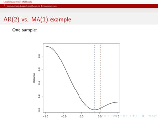
AR(2) vs. MA(1) example
true (AR) model
yt = t −θ t−1
and [wrong!] auxiliary (MA) model
yt = β1 yt−1 + β2 yt−2 + ut
R code
x=eps=rnorm(250)
x[2:250]=x[2:250]-0.5*x[1:249]
simeps=rnorm(250)
propeta=seq(-.99,.99,le=199)
dist=rep(0,199)
bethat=as.vector(arima(x,c(2,0,0),incl=FALSE)$coef)
for (t in 1:199)
dist[t]=sum((as.vector(arima(c(simeps[1],simeps[2:250]-propeta[t]*
simeps[1:249]),c(2,0,0),incl=FALSE)$coef)-bethat)^2)](https://image.slidesharecdn.com/romabc-120120013357-phpapp02/85/ABC-in-Roma-58-320.jpg)

![Likelihood-free Methods
simulation-based methods in Econometrics
Choice of pseudo-model
Pick model such that
ˆ
1. β(θ) not flat
(i.e. sensitive to changes in θ)
ˆ
2. β(θ) not dispersed (i.e. robust agains changes in ys (θ))
[Frigessi & Heggland, 2004]](https://image.slidesharecdn.com/romabc-120120013357-phpapp02/85/ABC-in-Roma-61-320.jpg)
![Likelihood-free Methods
simulation-based methods in Econometrics
ABC using indirect inference
We present a novel approach for developing summary statistics
for use in approximate Bayesian computation (ABC) algorithms by
using indirect inference(...) In the indirect inference approach to
ABC the parameters of an auxiliary model fitted to the data become
the summary statistics. Although applicable to any ABC technique,
we embed this approach within a sequential Monte Carlo algorithm
that is completely adaptive and requires very little tuning(...)
[Drovandi, Pettitt & Faddy, 2011]
c Indirect inference provides summary statistics for ABC...](https://image.slidesharecdn.com/romabc-120120013357-phpapp02/85/ABC-in-Roma-62-320.jpg)
![Likelihood-free Methods
simulation-based methods in Econometrics
ABC using indirect inference
...the above result shows that, in the limit as h → 0, ABC will
be more accurate than an indirect inference method whose auxiliary
statistics are the same as the summary statistic that is used for
ABC(...) Initial analysis showed that which method is more
accurate depends on the true value of θ.
[Fearnhead and Prangle, 2012]
c Indirect inference provides estimates rather than global inference...](https://image.slidesharecdn.com/romabc-120120013357-phpapp02/85/ABC-in-Roma-63-320.jpg)
![Likelihood-free Methods
Genetics of ABC
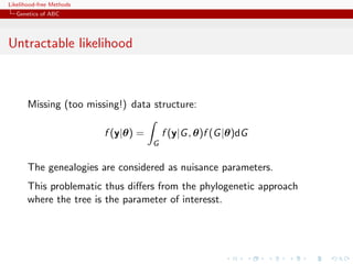
Genetic background of ABC
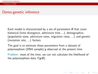
ABC is a recent computational technique that only requires being
able to sample from the likelihood f (·|θ)
This technique stemmed from population genetics models, about
15 years ago, and population geneticists still contribute
significantly to methodological developments of ABC.
[Griffith & al., 1997; Tavar´ & al., 1999]
e](https://image.slidesharecdn.com/romabc-120120013357-phpapp02/85/ABC-in-Roma-64-320.jpg)
![Likelihood-free Methods
Genetics of ABC
Population genetics
[Part derived from the teaching material of Raphael Leblois, ENS Lyon, November 2010]
Describe the genotypes, estimate the alleles frequencies,
determine their distribution among individuals, populations
and between populations;
Predict and understand the evolution of gene frequencies in
populations as a result of various factors.
c Analyses the effect of various evolutive forces (mutation, drift,
migration, selection) on the evolution of gene frequencies in time
and space.](https://image.slidesharecdn.com/romabc-120120013357-phpapp02/85/ABC-in-Roma-65-320.jpg)
![Likelihood-free Methods
Genetics of ABC
A[B]ctors
Les mécanismes de l’évolution
Towards an explanation of the mechanisms of evolutionary
changes, mathematical models ofl’évolution ont to be developed
•! Les mathématiques de evolution started
in the years 1920-1930.
commencé à être développés dans les
années 1920-1930
Ronald A Fisher (1890-1962) Sewall Wright (1889-1988) John BS Haldane (1892-1964)](https://image.slidesharecdn.com/romabc-120120013357-phpapp02/85/ABC-in-Roma-66-320.jpg)

![Likelihood-free Methods
Genetics of ABC
Coalescent theory
[Kingman, 1982; Tajima, Tavar´, &tc]
e
!"#$%&'(('")**+$,-'".'"/010234%'".'5"*$*%()23$15"6"
Coalescence theory interested in the genealogy of a sample of
!!7**+$,-'",()5534%'" common ancestor of the sample.
"
genes back in time to the " "!"7**+$,-'"8",$)('5,'1,'"9"](https://image.slidesharecdn.com/romabc-120120013357-phpapp02/85/ABC-in-Roma-68-320.jpg)


![Likelihood-free Methods
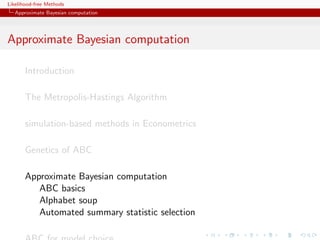
Approximate Bayesian computation
ABC basics
Illustrations
Example
Inference on CMB: in cosmology, study of the Cosmic Microwave
Background via likelihoods immensely slow to computate (e.g
WMAP, Plank), because of numerically costly spectral transforms
[Data is a Fortran program]
[Kilbinger et al., 2010, MNRAS]](https://image.slidesharecdn.com/romabc-120120013357-phpapp02/85/ABC-in-Roma-82-320.jpg)
![Likelihood-free Methods
Approximate Bayesian computation
ABC basics
Illustrations
Example
Phylogenetic tree: in population
genetics, reconstitution of a common
ancestor from a sample of genes via
a phylogenetic tree that is close to
impossible to integrate out
[100 processor days with 4
parameters]
[Cornuet et al., 2009, Bioinformatics]](https://image.slidesharecdn.com/romabc-120120013357-phpapp02/85/ABC-in-Roma-83-320.jpg)


![Likelihood-free Methods
Approximate Bayesian computation
ABC basics
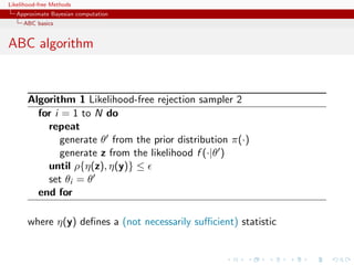
The ABC method
Bayesian setting: target is π(θ)f (x|θ)
When likelihood f (x|θ) not in closed form, likelihood-free rejection
technique:
ABC algorithm
For an observation y ∼ f (y|θ), under the prior π(θ), keep jointly
simulating
θ ∼ π(θ) , z ∼ f (z|θ ) ,
until the auxiliary variable z is equal to the observed value, z = y.
[Tavar´ et al., 1997]
e](https://image.slidesharecdn.com/romabc-120120013357-phpapp02/85/ABC-in-Roma-86-320.jpg)
![Likelihood-free Methods
Approximate Bayesian computation
ABC basics
Why does it work?!
The proof is trivial:
f (θi ) ∝ π(θi )f (z|θi )Iy (z)
z∈D
∝ π(θi )f (y|θi )
= π(θi |y) .
[Accept–Reject 101]](https://image.slidesharecdn.com/romabc-120120013357-phpapp02/85/ABC-in-Roma-87-320.jpg)
![Likelihood-free Methods
Approximate Bayesian computation
ABC basics
Earlier occurrence
‘Bayesian statistics and Monte Carlo methods are ideally
suited to the task of passing many models over one
dataset’
[Don Rubin, Annals of Statistics, 1984]
Note Rubin (1984) does not promote this algorithm for
likelihood-free simulation but frequentist intuition on posterior
distributions: parameters from posteriors are more likely to be
those that could have generated the data.](https://image.slidesharecdn.com/romabc-120120013357-phpapp02/85/ABC-in-Roma-88-320.jpg)

![Likelihood-free Methods
Approximate Bayesian computation
ABC basics
A as A...pproximative
When y is a continuous random variable, equality z = y is replaced
with a tolerance condition,
(y, z) ≤
where is a distance
Output distributed from
π(θ) Pθ { (y, z) < } ∝ π(θ| (y, z) < )
[Pritchard et al., 1999]](https://image.slidesharecdn.com/romabc-120120013357-phpapp02/85/ABC-in-Roma-90-320.jpg)


![Likelihood-free Methods
Approximate Bayesian computation
ABC basics
Convergence of ABC (first attempt)
What happens when → 0?
If f (·|θ) is continuous in y , uniformly in θ [!], given an arbitrary
δ > 0, there exists 0 such that < 0 implies
π(θ) f (z|θ)IA ,y (z) dz π(θ)f (y|θ)(1 δ)µ(B )
∈
A ,y ×Θ π(θ)f (z|θ)dzdθ Θ π(θ)f (y|θ)dθ(1 ± δ)µ(B )](https://image.slidesharecdn.com/romabc-120120013357-phpapp02/85/ABC-in-Roma-95-320.jpg)
![Likelihood-free Methods
Approximate Bayesian computation
ABC basics
Convergence of ABC (first attempt)
What happens when → 0?
If f (·|θ) is continuous in y , uniformly in θ [!], given an arbitrary
δ > 0, there exists 0 such that < 0 implies
π(θ) f (z|θ)IA ,y (z) dz π(θ)f (y|θ)(1 δ)
XX )
µ(BX
∈
A ,y ×Θ π(θ)f (z|θ)dzdθ Θ π(θ)f (y|θ)dθ(1 ± δ)
µ(B )
XXX](https://image.slidesharecdn.com/romabc-120120013357-phpapp02/85/ABC-in-Roma-96-320.jpg)
![Likelihood-free Methods
Approximate Bayesian computation
ABC basics
Convergence of ABC (first attempt)
What happens when → 0?
If f (·|θ) is continuous in y , uniformly in θ [!], given an arbitrary
δ 0, there exists 0 such that 0 implies
π(θ) f (z|θ)IA ,y (z) dz π(θ)f (y|θ)(1 δ)
XX )
µ(BX
∈
A ,y ×Θ π(θ)f (z|θ)dzdθ Θ π(θ)f (y|θ)dθ(1 ± δ) X
µ(B )
X
X
[Proof extends to other continuous-in-0 kernels K ]](https://image.slidesharecdn.com/romabc-120120013357-phpapp02/85/ABC-in-Roma-97-320.jpg)


![Likelihood-free Methods
Approximate Bayesian computation
ABC basics
MA example
Back to the MA(q) model
q
xt = t + ϑi t−i
i=1
Simple prior: uniform over the inverse [real and complex] roots in
q
Q(u) = 1 − ϑi u i
i=1
under the identifiability conditions](https://image.slidesharecdn.com/romabc-120120013357-phpapp02/85/ABC-in-Roma-105-320.jpg)


![Likelihood-free Methods
Approximate Bayesian computation
ABC basics
Homonomy
The ABC algorithm is not to be confused with the ABC algorithm
The Artificial Bee Colony algorithm is a swarm based meta-heuristic
algorithm that was introduced by Karaboga in 2005 for optimizing
numerical problems. It was inspired by the intelligent foraging
behavior of honey bees. The algorithm is specifically based on the
model proposed by Tereshko and Loengarov (2005) for the foraging
behaviour of honey bee colonies. The model consists of three
essential components: employed and unemployed foraging bees, and
food sources. The first two components, employed and unemployed
foraging bees, search for rich food sources (...) close to their hive.
The model also defines two leading modes of behaviour (...):
recruitment of foragers to rich food sources resulting in positive
feedback and abandonment of poor sources by foragers causing
negative feedback.
[Karaboga, Scholarpedia]](https://image.slidesharecdn.com/romabc-120120013357-phpapp02/85/ABC-in-Roma-112-320.jpg)

![Likelihood-free Methods
Approximate Bayesian computation
ABC basics
ABC advances
Simulating from the prior is often poor in efficiency
Either modify the proposal distribution on θ to increase the density
of x’s within the vicinity of y ...
[Marjoram et al, 2003; Bortot et al., 2007, Sisson et al., 2007]](https://image.slidesharecdn.com/romabc-120120013357-phpapp02/85/ABC-in-Roma-114-320.jpg)
![Likelihood-free Methods
Approximate Bayesian computation
ABC basics
ABC advances
Simulating from the prior is often poor in efficiency
Either modify the proposal distribution on θ to increase the density
of x’s within the vicinity of y ...
[Marjoram et al, 2003; Bortot et al., 2007, Sisson et al., 2007]
...or by viewing the problem as a conditional density estimation
and by developing techniques to allow for larger
[Beaumont et al., 2002]](https://image.slidesharecdn.com/romabc-120120013357-phpapp02/85/ABC-in-Roma-115-320.jpg)
![Likelihood-free Methods
Approximate Bayesian computation
ABC basics
ABC advances
Simulating from the prior is often poor in efficiency
Either modify the proposal distribution on θ to increase the density
of x’s within the vicinity of y ...
[Marjoram et al, 2003; Bortot et al., 2007, Sisson et al., 2007]
...or by viewing the problem as a conditional density estimation
and by developing techniques to allow for larger
[Beaumont et al., 2002]
.....or even by including in the inferential framework [ABCµ ]
[Ratmann et al., 2009]](https://image.slidesharecdn.com/romabc-120120013357-phpapp02/85/ABC-in-Roma-116-320.jpg)
![Likelihood-free Methods
Approximate Bayesian computation
Alphabet soup
ABC-NP
Better usage of [prior] simulations by
adjustement: instead of throwing away
θ such that ρ(η(z), η(y)) , replace
θ’s with locally regressed transforms
(use with BIC)
θ∗ = θ − {η(z) − η(y)}T β
ˆ [Csill´ry et al., TEE, 2010]
e
ˆ
where β is obtained by [NP] weighted least square regression on
(η(z) − η(y)) with weights
Kδ {ρ(η(z), η(y))}
[Beaumont et al., 2002, Genetics]](https://image.slidesharecdn.com/romabc-120120013357-phpapp02/85/ABC-in-Roma-117-320.jpg)
![Likelihood-free Methods
Approximate Bayesian computation
Alphabet soup
ABC-NP (regression)
Also found in the subsequent literature, e.g. in Fearnhead-Prangle (2012) :
weight directly simulation by
Kδ {ρ(η(z(θ)), η(y))}
or
S
1
Kδ {ρ(η(zs (θ)), η(y))}
S
s=1
[consistent estimate of f (η|θ)]](https://image.slidesharecdn.com/romabc-120120013357-phpapp02/85/ABC-in-Roma-118-320.jpg)
![Likelihood-free Methods
Approximate Bayesian computation
Alphabet soup
ABC-NP (regression)
Also found in the subsequent literature, e.g. in Fearnhead-Prangle (2012) :
weight directly simulation by
Kδ {ρ(η(z(θ)), η(y))}
or
S
1
Kδ {ρ(η(zs (θ)), η(y))}
S
s=1
[consistent estimate of f (η|θ)]
Curse of dimensionality: poor estimate when d = dim(η) is large...](https://image.slidesharecdn.com/romabc-120120013357-phpapp02/85/ABC-in-Roma-119-320.jpg)
![Likelihood-free Methods
Approximate Bayesian computation
Alphabet soup
ABC-NP (density estimation)
Use of the kernel weights
Kδ {ρ(η(z(θ)), η(y))}
leads to the NP estimate of the posterior expectation
i θi Kδ {ρ(η(z(θi )), η(y))}
i Kδ {ρ(η(z(θi )), η(y))}
[Blum, JASA, 2010]](https://image.slidesharecdn.com/romabc-120120013357-phpapp02/85/ABC-in-Roma-120-320.jpg)
![Likelihood-free Methods
Approximate Bayesian computation
Alphabet soup
ABC-NP (density estimation)
Use of the kernel weights
Kδ {ρ(η(z(θ)), η(y))}
leads to the NP estimate of the posterior conditional density
˜
Kb (θi − θ)Kδ {ρ(η(z(θi )), η(y))}
i
i Kδ {ρ(η(z(θi )), η(y))}
[Blum, JASA, 2010]](https://image.slidesharecdn.com/romabc-120120013357-phpapp02/85/ABC-in-Roma-121-320.jpg)

![Likelihood-free Methods
Approximate Bayesian computation
Alphabet soup
ABC-NP (density estimations)
Other versions incorporating regression adjustments
˜
Kb (θi∗ − θ)Kδ {ρ(η(z(θi )), η(y))}
i
i Kδ {ρ(η(z(θi )), η(y))}
In all cases, error
E[ˆ (θ|y)] − g (θ|y) = cb 2 + cδ 2 + OP (b 2 + δ 2 ) + OP (1/nδ d )
g
c
var(ˆ (θ|y)) =
g (1 + oP (1))
nbδ d
[Blum, JASA, 2010]](https://image.slidesharecdn.com/romabc-120120013357-phpapp02/85/ABC-in-Roma-123-320.jpg)
![Likelihood-free Methods
Approximate Bayesian computation
Alphabet soup
ABC-NP (density estimations)
Other versions incorporating regression adjustments
˜
Kb (θi∗ − θ)Kδ {ρ(η(z(θi )), η(y))}
i
i Kδ {ρ(η(z(θi )), η(y))}
In all cases, error
E[ˆ (θ|y)] − g (θ|y) = cb 2 + cδ 2 + OP (b 2 + δ 2 ) + OP (1/nδ d )
g
c
var(ˆ (θ|y)) =
g (1 + oP (1))
nbδ d
[standard NP calculations]](https://image.slidesharecdn.com/romabc-120120013357-phpapp02/85/ABC-in-Roma-124-320.jpg)
![Likelihood-free Methods
Approximate Bayesian computation
Alphabet soup
ABC-NCH
Incorporating non-linearities and heterocedasticities:
σ (η(y))
ˆ
θ∗ = m(η(y)) + [θ − m(η(z))]
ˆ ˆ
σ (η(z))
ˆ](https://image.slidesharecdn.com/romabc-120120013357-phpapp02/85/ABC-in-Roma-125-320.jpg)
![Likelihood-free Methods
Approximate Bayesian computation
Alphabet soup
ABC-NCH
Incorporating non-linearities and heterocedasticities:
σ (η(y))
ˆ
θ∗ = m(η(y)) + [θ − m(η(z))]
ˆ ˆ
σ (η(z))
ˆ
where
m(η) estimated by non-linear regression (e.g., neural network)
ˆ
σ (η) estimated by non-linear regression on residuals
ˆ
log{θi − m(ηi )}2 = log σ 2 (ηi ) + ξi
ˆ
[Blum Fran¸ois, 2009]
c](https://image.slidesharecdn.com/romabc-120120013357-phpapp02/85/ABC-in-Roma-126-320.jpg)

![Likelihood-free Methods
Approximate Bayesian computation
Alphabet soup
ABC-NCH (2)
Why neural network?
fights curse of dimensionality
selects relevant summary statistics
provides automated dimension reduction
offers a model choice capability
improves upon multinomial logistic
[Blum Fran¸ois, 2009]
c](https://image.slidesharecdn.com/romabc-120120013357-phpapp02/85/ABC-in-Roma-128-320.jpg)
![Likelihood-free Methods
Approximate Bayesian computation
Alphabet soup
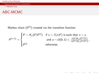
ABC-MCMC
Markov chain (θ(t) ) created via the transition function
θ ∼ Kω (θ |θ(t) ) if x ∼ f (x|θ ) is such that x = y
π(θ )Kω (t) |θ )
θ (t+1)
= and u ∼ U(0, 1) ≤ π(θ(t) )K (θ |θ(t) ) ,
ω (θ
(t)
θ otherwise,
has the posterior π(θ|y ) as stationary distribution
[Marjoram et al, 2003]](https://image.slidesharecdn.com/romabc-120120013357-phpapp02/85/ABC-in-Roma-130-320.jpg)
![Likelihood-free Methods
Approximate Bayesian computation
Alphabet soup
ABC-MCMC (2)
Algorithm 2 Likelihood-free MCMC sampler
Use Algorithm 1 to get (θ(0) , z(0) )
for t = 1 to N do
Generate θ from Kω ·|θ(t−1) ,
Generate z from the likelihood f (·|θ ),
Generate u from U[0,1] ,
π(θ )Kω (θ(t−1) |θ )
if u ≤ I
π(θ(t−1) Kω (θ |θ(t−1) ) A ,y (z ) then
set (θ(t) , z(t) ) = (θ , z )
else
(θ(t) , z(t) )) = (θ(t−1) , z(t−1) ),
end if
end for](https://image.slidesharecdn.com/romabc-120120013357-phpapp02/85/ABC-in-Roma-131-320.jpg)


![Likelihood-free Methods
Approximate Bayesian computation
Alphabet soup
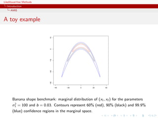
A toy example
Case of
1 1
x ∼ N (θ, 1) + N (θ, 1)
2 2
under prior θ ∼ N (0, 10)
ABC sampler
thetas=rnorm(N,sd=10)
zed=sample(c(1,-1),N,rep=TRUE)*thetas+rnorm(N,sd=1)
eps=quantile(abs(zed-x),.01)
abc=thetas[abs(zed-x)eps]](https://image.slidesharecdn.com/romabc-120120013357-phpapp02/85/ABC-in-Roma-136-320.jpg)
![Likelihood-free Methods
Approximate Bayesian computation
Alphabet soup
A toy example
Case of
1 1
x ∼ N (θ, 1) + N (θ, 1)
2 2
under prior θ ∼ N (0, 10)
ABC-MCMC sampler
metas=rep(0,N)
metas[1]=rnorm(1,sd=10)
zed[1]=x
for (t in 2:N){
metas[t]=rnorm(1,mean=metas[t-1],sd=5)
zed[t]=rnorm(1,mean=(1-2*(runif(1).5))*metas[t],sd=1)
if ((abs(zed[t]-x)eps)||(runif(1)dnorm(metas[t],sd=10)/dnorm(metas[t-1],sd=10))){
metas[t]=metas[t-1]
zed[t]=zed[t-1]}
}](https://image.slidesharecdn.com/romabc-120120013357-phpapp02/85/ABC-in-Roma-137-320.jpg)


![Likelihood-free Methods
Approximate Bayesian computation
Alphabet soup
ABCµ
[Ratmann, Andrieu, Wiuf and Richardson, 2009, PNAS]
Use of a joint density
f (θ, |y) ∝ ξ( |y, θ) × πθ (θ) × π ( )
where y is the data, and ξ( |y, θ) is the prior predictive density of
ρ(η(z), η(y)) given θ and x when z ∼ f (z|θ)](https://image.slidesharecdn.com/romabc-120120013357-phpapp02/85/ABC-in-Roma-144-320.jpg)
![Likelihood-free Methods
Approximate Bayesian computation
Alphabet soup
ABCµ
[Ratmann, Andrieu, Wiuf and Richardson, 2009, PNAS]
Use of a joint density
f (θ, |y) ∝ ξ( |y, θ) × πθ (θ) × π ( )
where y is the data, and ξ( |y, θ) is the prior predictive density of
ρ(η(z), η(y)) given θ and x when z ∼ f (z|θ)
Warning! Replacement of ξ( |y, θ) with a non-parametric kernel
approximation.](https://image.slidesharecdn.com/romabc-120120013357-phpapp02/85/ABC-in-Roma-145-320.jpg)
![Likelihood-free Methods
Approximate Bayesian computation
Alphabet soup
ABCµ details
Multidimensional distances ρk (k = 1, . . . , K ) and errors
k = ρk (ηk (z), ηk (y)), with
ˆ 1
k ∼ ξk ( |y, θ) ≈ ξk ( |y, θ) = K [{ k −ρk (ηk (zb ), ηk (y))}/hk ]
Bhk
b
ˆ
then used in replacing ξ( |y, θ) with mink ξk ( |y, θ)](https://image.slidesharecdn.com/romabc-120120013357-phpapp02/85/ABC-in-Roma-146-320.jpg)
![Likelihood-free Methods
Approximate Bayesian computation
Alphabet soup
ABCµ details
Multidimensional distances ρk (k = 1, . . . , K ) and errors
k = ρk (ηk (z), ηk (y)), with
ˆ 1
k ∼ ξk ( |y, θ) ≈ ξk ( |y, θ) = K [{ k −ρk (ηk (zb ), ηk (y))}/hk ]
Bhk
b
ˆ
then used in replacing ξ( |y, θ) with mink ξk ( |y, θ)
ABCµ involves acceptance probability
ˆ
π(θ , ) q(θ , θ)q( , ) mink ξk ( |y, θ )
ˆ
π(θ, ) q(θ, θ )q( , ) mink ξk ( |y, θ)](https://image.slidesharecdn.com/romabc-120120013357-phpapp02/85/ABC-in-Roma-147-320.jpg)
![Likelihood-free Methods
Approximate Bayesian computation
Alphabet soup
ABCµ multiple errors
[ c Ratmann et al., PNAS, 2009]](https://image.slidesharecdn.com/romabc-120120013357-phpapp02/85/ABC-in-Roma-148-320.jpg)
![Likelihood-free Methods
Approximate Bayesian computation
Alphabet soup
ABCµ for model choice
[ c Ratmann et al., PNAS, 2009]](https://image.slidesharecdn.com/romabc-120120013357-phpapp02/85/ABC-in-Roma-149-320.jpg)

![Likelihood-free Methods
Approximate Bayesian computation
Alphabet soup
Questions about ABCµ
For each model under comparison, marginal posterior on used to
assess the fit of the model (HPD includes 0 or not).
Is the data informative about ? [Identifiability]
How is the prior π( ) impacting the comparison?
How is using both ξ( |x0 , θ) and π ( ) compatible with a
standard probability model? [remindful of Wilkinson ]
Where is the penalisation for complexity in the model
comparison?
[X, Mengersen Chen, 2010, PNAS]](https://image.slidesharecdn.com/romabc-120120013357-phpapp02/85/ABC-in-Roma-151-320.jpg)

![Likelihood-free Methods
Approximate Bayesian computation
Alphabet soup
ABC-PRC
Another sequential version producing a sequence of Markov
(t) (t)
transition kernels Kt and of samples (θ1 , . . . , θN ) (1 ≤ t ≤ T )
ABC-PRC Algorithm
(t−1)
1. Select θ at random from previous θi ’s with probabilities
(t−1)
ωi (1 ≤ i ≤ N).
2. Generate
(t) (t)
θi ∼ Kt (θ|θ ) , x ∼ f (x|θi ) ,
3. Check that (x, y ) , otherwise start again.
[Sisson et al., 2007]](https://image.slidesharecdn.com/romabc-120120013357-phpapp02/85/ABC-in-Roma-153-320.jpg)
![Likelihood-free Methods
Approximate Bayesian computation
Alphabet soup
Why PRC?
Partial rejection control: Resample from a population of weighted
particles by pruning away particles with weights below threshold C ,
replacing them by new particles obtained by propagating an
existing particle by an SMC step and modifying the weights
accordinly.
[Liu, 2001]](https://image.slidesharecdn.com/romabc-120120013357-phpapp02/85/ABC-in-Roma-154-320.jpg)
![Likelihood-free Methods
Approximate Bayesian computation
Alphabet soup
Why PRC?
Partial rejection control: Resample from a population of weighted
particles by pruning away particles with weights below threshold C ,
replacing them by new particles obtained by propagating an
existing particle by an SMC step and modifying the weights
accordinly.
[Liu, 2001]
PRC justification in ABC-PRC:
Suppose we then implement the PRC algorithm for some
c 0 such that only identically zero weights are smaller
than c
Trouble is, there is no such c...](https://image.slidesharecdn.com/romabc-120120013357-phpapp02/85/ABC-in-Roma-155-320.jpg)


![Likelihood-free Methods
Approximate Bayesian computation
Alphabet soup
ABC-PRC bias
Lack of unbiasedness of the method
Joint density of the accepted pair (θ(t−1) , θ(t) ) proportional to
(t−1) (t) (t−1) (t)
π(θ |y )Kt (θ |θ )f (y |θ ),
For an arbitrary function h(θ), E [ωt h(θ(t) )] proportional to
(t) π(θ (t) )Lt−1 (θ (t−1) |θ (t) ) (t−1) (t) (t−1) (t) (t−1) (t)
h(θ ) π(θ |y )Kt (θ |θ )f (y |θ )dθ dθ
π(θ (t−1) )Kt (θ (t) |θ (t−1) )
(t) π(θ (t) )Lt−1 (θ (t−1) |θ (t) ) (t−1) (t−1)
∝ h(θ ) π(θ )f (y |θ )
π(θ (t−1) )Kt (θ (t) |θ (t−1) )
(t) (t−1) (t) (t−1) (t)
× Kt (θ |θ )f (y |θ )dθ dθ
(t) (t) (t−1) (t) (t−1) (t−1) (t)
∝ h(θ )π(θ |y ) Lt−1 (θ |θ )f (y |θ )dθ dθ .](https://image.slidesharecdn.com/romabc-120120013357-phpapp02/85/ABC-in-Roma-160-320.jpg)
![Likelihood-free Methods
Approximate Bayesian computation
Alphabet soup
A mixture example (1)
Toy model of Sisson et al. (2007): if
θ ∼ U(−10, 10) , x|θ ∼ 0.5 N (θ, 1) + 0.5 N (θ, 1/100) ,
then the posterior distribution associated with y = 0 is the normal
mixture
θ|y = 0 ∼ 0.5 N (0, 1) + 0.5 N (0, 1/100)
restricted to [−10, 10].
Furthermore, true target available as
π(θ||x| ) ∝ Φ( −θ)−Φ(− −θ)+Φ(10( −θ))−Φ(−10( +θ)) .](https://image.slidesharecdn.com/romabc-120120013357-phpapp02/85/ABC-in-Roma-161-320.jpg)

![Likelihood-free Methods
Approximate Bayesian computation
Alphabet soup
A PMC version
Use of the same kernel idea as ABC-PRC but with IS correction
( check PMC )
Generate a sample at iteration t by
N
(t) (t−1) (t−1)
πt (θ
ˆ )∝ ωj Kt (θ(t) |θj )
j=1
modulo acceptance of the associated xt , and use an importance
(t)
weight associated with an accepted simulation θi
(t) (t) (t)
ωi ∝ π(θi ) πt (θi ) .
ˆ
c Still likelihood free
[Beaumont et al., 2009]](https://image.slidesharecdn.com/romabc-120120013357-phpapp02/85/ABC-in-Roma-163-320.jpg)

![Likelihood-free Methods
Approximate Bayesian computation
Alphabet soup
Sequential Monte Carlo
SMC is a simulation technique to approximate a sequence of
related probability distributions πn with π0 “easy” and πT as
target.
Iterated IS as PMC: particles moved from time n to time n via
kernel Kn and use of a sequence of extended targets πn˜
n
πn (z0:n ) = πn (zn )
˜ Lj (zj+1 , zj )
j=0
where the Lj ’s are backward Markov kernels [check that πn (zn ) is a
marginal]
[Del Moral, Doucet Jasra, Series B, 2006]](https://image.slidesharecdn.com/romabc-120120013357-phpapp02/85/ABC-in-Roma-165-320.jpg)
![Likelihood-free Methods
Approximate Bayesian computation
Alphabet soup
ABC-SMC
[Del Moral, Doucet Jasra, 2009]
True derivation of an SMC-ABC algorithm
Use of a kernel Kn associated with target π n and derivation of the
backward kernel
π n (z )Kn (z , z)
Ln−1 (z, z ) =
πn (z)
Update of the weights
M m
m=1 IA n
(xin )
win ∝ wi(n−1) M m
(xi(n−1) )
m=1 IA n−1
m
when xin ∼ K (xi(n−1) , ·)](https://image.slidesharecdn.com/romabc-120120013357-phpapp02/85/ABC-in-Roma-167-320.jpg)
![Likelihood-free Methods
Approximate Bayesian computation
Alphabet soup
ABC-SMCM
Modification: Makes M repeated simulations of the pseudo-data z
given the parameter, rather than using a single [M = 1] simulation,
leading to weight that is proportional to the number of accepted
zi s
M
1
ω(θ) = Iρ(η(y),η(zi ))
M
i=1
[limit in M means exact simulation from (tempered) target]](https://image.slidesharecdn.com/romabc-120120013357-phpapp02/85/ABC-in-Roma-168-320.jpg)
![Likelihood-free Methods
Approximate Bayesian computation
Alphabet soup
Properties of ABC-SMC
The ABC-SMC method properly uses a backward kernel L(z, z ) to
simplify the importance weight and to remove the dependence on
the unknown likelihood from this weight. Update of importance
weights is reduced to the ratio of the proportions of surviving
particles
Major assumption: the forward kernel K is supposed to be invariant
against the true target [tempered version of the true posterior]](https://image.slidesharecdn.com/romabc-120120013357-phpapp02/85/ABC-in-Roma-169-320.jpg)
![Likelihood-free Methods
Approximate Bayesian computation
Alphabet soup
Properties of ABC-SMC
The ABC-SMC method properly uses a backward kernel L(z, z ) to
simplify the importance weight and to remove the dependence on
the unknown likelihood from this weight. Update of importance
weights is reduced to the ratio of the proportions of surviving
particles
Major assumption: the forward kernel K is supposed to be invariant
against the true target [tempered version of the true posterior]
Adaptivity in ABC-SMC algorithm only found in on-line
construction of the thresholds t , slowly enough to keep a large
number of accepted transitions](https://image.slidesharecdn.com/romabc-120120013357-phpapp02/85/ABC-in-Roma-170-320.jpg)

![Likelihood-free Methods
Approximate Bayesian computation
Alphabet soup
Yet another ABC-PRC
Another version of ABC-PRC called PRC-ABC with a proposal
distribution Mt , S replications of the pseudo-data, and a PRC step:
PRC-ABC Algorithm
(t−1) (t−1)
1. Select θ at random from the θi ’s with probabilities ωi
(t) iid (t−1)
2. Generate θi ∼ Kt , x1 , . . . , xS ∼ f (x|θi ), set
(t) (t)
ωi = Kt {η(xs ) − η(y)} Kt (θi ) ,
s
(t)
and accept with probability p (i) = ωi /ct,N
(t) (t)
3. Set ωi ∝ ωi /p (i) (1 ≤ i ≤ N)
[Peters, Sisson Fan, Stat Computing, 2012]](https://image.slidesharecdn.com/romabc-120120013357-phpapp02/85/ABC-in-Roma-172-320.jpg)

![Likelihood-free Methods
Approximate Bayesian computation
Alphabet soup
Wilkinson’s exact BC
ABC approximation error (i.e. non-zero tolerance) replaced with
exact simulation from a controlled approximation to the target,
convolution of true posterior with kernel function
π(θ)f (z|θ)K (y − z)
π (θ, z|y) = ,
π(θ)f (z|θ)K (y − z)dzdθ
with K kernel parameterised by bandwidth .
[Wilkinson, 2008]](https://image.slidesharecdn.com/romabc-120120013357-phpapp02/85/ABC-in-Roma-174-320.jpg)
![Likelihood-free Methods
Approximate Bayesian computation
Alphabet soup
Wilkinson’s exact BC
ABC approximation error (i.e. non-zero tolerance) replaced with
exact simulation from a controlled approximation to the target,
convolution of true posterior with kernel function
π(θ)f (z|θ)K (y − z)
π (θ, z|y) = ,
π(θ)f (z|θ)K (y − z)dzdθ
with K kernel parameterised by bandwidth .
[Wilkinson, 2008]
Theorem
The ABC algorithm based on the assumption of a randomised
observation y = y + ξ, ξ ∼ K , and an acceptance probability of
˜
K (y − z)/M
gives draws from the posterior distribution π(θ|y).](https://image.slidesharecdn.com/romabc-120120013357-phpapp02/85/ABC-in-Roma-175-320.jpg)
![Likelihood-free Methods
Approximate Bayesian computation
Alphabet soup
How exact a BC?
“Using to represent measurement error is
straightforward, whereas using to model the model
discrepancy is harder to conceptualize and not as
commonly used”
[Richard Wilkinson, 2008]](https://image.slidesharecdn.com/romabc-120120013357-phpapp02/85/ABC-in-Roma-176-320.jpg)
![Likelihood-free Methods
Approximate Bayesian computation
Alphabet soup
How exact a BC?
Pros
Pseudo-data from true model and observed data from noisy
model
Interesting perspective in that outcome is completely
controlled
Link with ABCµ and assuming y is observed with a
measurement error with density K
Relates to the theory of model approximation
[Kennedy O’Hagan, 2001]
Cons
Requires K to be bounded by M
True approximation error never assessed
Requires a modification of the standard ABC algorithm](https://image.slidesharecdn.com/romabc-120120013357-phpapp02/85/ABC-in-Roma-177-320.jpg)
![Likelihood-free Methods
Approximate Bayesian computation
Alphabet soup
ABC for HMMs
Specific case of a hidden Markov model
Xt+1 ∼ Qθ (Xt , ·)
Yt+1 ∼ gθ (·|xt )
0
where only y1:n is observed.
[Dean, Singh, Jasra, Peters, 2011]](https://image.slidesharecdn.com/romabc-120120013357-phpapp02/85/ABC-in-Roma-178-320.jpg)
![Likelihood-free Methods
Approximate Bayesian computation
Alphabet soup
ABC for HMMs
Specific case of a hidden Markov model
Xt+1 ∼ Qθ (Xt , ·)
Yt+1 ∼ gθ (·|xt )
0
where only y1:n is observed.
[Dean, Singh, Jasra, Peters, 2011]
Use of specific constraints, adapted to the Markov structure:
0 0
y1 ∈ B(y1 , ) × · · · × yn ∈ B(yn , )](https://image.slidesharecdn.com/romabc-120120013357-phpapp02/85/ABC-in-Roma-179-320.jpg)

![Likelihood-free Methods
Approximate Bayesian computation
Alphabet soup
ABC-MLE for HMMs
ABC-MLE defined by
ˆ 0 0
θn = arg max Pθ Y1 ∈ B(y1 , ), . . . , Yn ∈ B(yn , )
θ
Exact MLE for the likelihood same basis as Wilkinson!
0
pθ (y1 , . . . , yn )
corresponding to the perturbed process
(xt , yt + zt )1≤t≤n zt ∼ U(B(0, 1)
[Dean, Singh, Jasra, Peters, 2011]](https://image.slidesharecdn.com/romabc-120120013357-phpapp02/85/ABC-in-Roma-181-320.jpg)
![Likelihood-free Methods
Approximate Bayesian computation
Alphabet soup
ABC-MLE is biased
ABC-MLE is asymptotically (in n) biased with target
l (θ) = Eθ∗ [log pθ (Y1 |Y−∞:0 )]](https://image.slidesharecdn.com/romabc-120120013357-phpapp02/85/ABC-in-Roma-182-320.jpg)
![Likelihood-free Methods
Approximate Bayesian computation
Alphabet soup
ABC-MLE is biased
ABC-MLE is asymptotically (in n) biased with target
l (θ) = Eθ∗ [log pθ (Y1 |Y−∞:0 )]
but ABD-MLE converges to true value in the sense
l n (θn ) → l (θ)
for all sequences (θn ) converging to θ and n](https://image.slidesharecdn.com/romabc-120120013357-phpapp02/85/ABC-in-Roma-183-320.jpg)
![Likelihood-free Methods
Approximate Bayesian computation
Alphabet soup
Noisy ABC-MLE
Idea: Modify instead the data from the start
0
(y1 + ζ1 , . . . , yn + ζn )
[ see Fearnhead-Prangle ]
noisy ABC-MLE estimate
0 0
arg max Pθ Y1 ∈ B(y1 + ζ1 , ), . . . , Yn ∈ B(yn + ζn , )
θ
[Dean, Singh, Jasra, Peters, 2011]](https://image.slidesharecdn.com/romabc-120120013357-phpapp02/85/ABC-in-Roma-184-320.jpg)

![Likelihood-free Methods
Approximate Bayesian computation
Alphabet soup
SMC for ABC likelihood
Algorithm 4 SMC ABC for HMMs
Given θ
for k = 1, . . . , n do
1 1 N N
generate proposals (xk , yk ), . . . , (xk , yk ) from the model
weigh each proposal with ωk l =I l
B(yk + ζk , ) (yk )
0
l
renormalise the weights and sample the xk ’s accordingly
end for
approximate the likelihood by
n N
l
ωk N
k=1 l=1
[Jasra, Singh, Martin, McCoy, 2010]](https://image.slidesharecdn.com/romabc-120120013357-phpapp02/85/ABC-in-Roma-186-320.jpg)
![Likelihood-free Methods
Approximate Bayesian computation
Alphabet soup
Which summary?
Fundamental difficulty of the choice of the summary statistic when
there is no non-trivial sufficient statistics [except when done by the
experimenters in the field]](https://image.slidesharecdn.com/romabc-120120013357-phpapp02/85/ABC-in-Roma-187-320.jpg)
![Likelihood-free Methods
Approximate Bayesian computation
Alphabet soup
Which summary?
Fundamental difficulty of the choice of the summary statistic when
there is no non-trivial sufficient statistics [except when done by the
experimenters in the field]
Starting from a large collection of summary statistics is available,
Joyce and Marjoram (2008) consider the sequential inclusion into
the ABC target, with a stopping rule based on a likelihood ratio
test.](https://image.slidesharecdn.com/romabc-120120013357-phpapp02/85/ABC-in-Roma-188-320.jpg)
![Likelihood-free Methods
Approximate Bayesian computation
Alphabet soup
Which summary?
Fundamental difficulty of the choice of the summary statistic when
there is no non-trivial sufficient statistics [except when done by the
experimenters in the field]
Starting from a large collection of summary statistics is available,
Joyce and Marjoram (2008) consider the sequential inclusion into
the ABC target, with a stopping rule based on a likelihood ratio
test.
Does not taking into account the sequential nature of the tests
Depends on parameterisation
Order of inclusion matters.](https://image.slidesharecdn.com/romabc-120120013357-phpapp02/85/ABC-in-Roma-189-320.jpg)
![Likelihood-free Methods
Approximate Bayesian computation
Alphabet soup
A connected Monte Carlo study
of the pseudo-data per simulated parameter
Repeating simulations
does not improve approximation
Tolerance level does not seem to be highly influential
Choice of distance / summary statistics / calibration factors
are paramount to successful approximation
ABC-SMC outperforms ABC-MCMC
[Mckinley, Cook, Deardon, 2009]](https://image.slidesharecdn.com/romabc-120120013357-phpapp02/85/ABC-in-Roma-190-320.jpg)

![Likelihood-free Methods
Approximate Bayesian computation
Automated summary statistic selection
Semi-automatic ABC
Fearnhead and Prangle (2010) study ABC and the selection of the
summary statistic in close proximity to Wilkinson’s proposal
ABC then considered from a purely inferential viewpoint and
calibrated for estimation purposes.
Use of a randomised (or ‘noisy’) version of the summary statistics
η (y) = η(y) + τ
˜
Derivation of a well-calibrated version of ABC, i.e. an algorithm
that gives proper predictions for the distribution associated with
this randomised summary statistic. [calibration constraint: ABC
approximation with same posterior mean as the true randomised
posterior.]](https://image.slidesharecdn.com/romabc-120120013357-phpapp02/85/ABC-in-Roma-192-320.jpg)
![Likelihood-free Methods
Approximate Bayesian computation
Automated summary statistic selection
Summary statistics
Optimality of the posterior expectation E[θ|y] of the parameter of
interest as summary statistics η(y)!](https://image.slidesharecdn.com/romabc-120120013357-phpapp02/85/ABC-in-Roma-193-320.jpg)
![Likelihood-free Methods
Approximate Bayesian computation
Automated summary statistic selection
Summary statistics
Optimality of the posterior expectation E[θ|y] of the parameter of
interest as summary statistics η(y)!
Use of the standard quadratic loss function
(θ − θ0 )T A(θ − θ0 ) .](https://image.slidesharecdn.com/romabc-120120013357-phpapp02/85/ABC-in-Roma-194-320.jpg)
![Likelihood-free Methods
Approximate Bayesian computation
Automated summary statistic selection
Details on Fearnhead and Prangle (FP) ABC
Use of a summary statistic S(·), an importance proposal g (·), a
kernel K (·) ≤ 1 and a bandwidth h 0 such that
(θ, ysim ) ∼ g (θ)f (ysim |θ)
is accepted with probability (hence the bound)
K [{S(ysim ) − sobs }/h]
and the corresponding importance weight defined by
π(θ) g (θ)
[Fearnhead Prangle, 2012]](https://image.slidesharecdn.com/romabc-120120013357-phpapp02/85/ABC-in-Roma-195-320.jpg)
![Likelihood-free Methods
Approximate Bayesian computation
Automated summary statistic selection
Errors, errors, and errors
Three levels of approximation
π(θ|yobs ) by π(θ|sobs ) loss of information
[ignored]
π(θ|sobs ) by
π(s)K [{s − sobs }/h]π(θ|s) ds
πABC (θ|sobs ) =
π(s)K [{s − sobs }/h] ds
noisy observations
πABC (θ|sobs ) by importance Monte Carlo based on N
simulations, represented by var(a(θ)|sobs )/Nacc [expected
number of acceptances]
[M. Twain/B. Disraeli]](https://image.slidesharecdn.com/romabc-120120013357-phpapp02/85/ABC-in-Roma-196-320.jpg)
![Likelihood-free Methods
Approximate Bayesian computation
Automated summary statistic selection
Average acceptance asymptotics
For the average acceptance probability/approximate likelihood
p(θ|sobs ) = f (ysim |θ) K [{S(ysim ) − sobs }/h] dysim ,
overall acceptance probability
p(sobs ) = p(θ|sobs ) π(θ) dθ = π(sobs )hd + o(hd )
[FP, Lemma 1]](https://image.slidesharecdn.com/romabc-120120013357-phpapp02/85/ABC-in-Roma-197-320.jpg)
![Likelihood-free Methods
Approximate Bayesian computation
Automated summary statistic selection
Optimal importance proposal
Best choice of importance proposal in terms of effective sample size
g (θ|sobs ) ∝ π(θ)p(θ|sobs )1/2
[Not particularly useful in practice]](https://image.slidesharecdn.com/romabc-120120013357-phpapp02/85/ABC-in-Roma-198-320.jpg)
![Likelihood-free Methods
Approximate Bayesian computation
Automated summary statistic selection
Optimal importance proposal
Best choice of importance proposal in terms of effective sample size
g (θ|sobs ) ∝ π(θ)p(θ|sobs )1/2
[Not particularly useful in practice]
note that p(θ|sobs ) is an approximate likelihood
reminiscent of parallel tempering
could be approximately achieved by attrition of half of the
data](https://image.slidesharecdn.com/romabc-120120013357-phpapp02/85/ABC-in-Roma-199-320.jpg)
![Likelihood-free Methods
Approximate Bayesian computation
Automated summary statistic selection
Calibration of h
“This result gives insight into how S(·) and h affect the Monte
Carlo error. To minimize Monte Carlo error, we need hd to be not
too small. Thus ideally we want S(·) to be a low dimensional
summary of the data that is sufficiently informative about θ that
π(θ|sobs ) is close, in some sense, to π(θ|yobs )” (FP, p.5)
turns h into an absolute value while it should be
context-dependent and user-calibrated
only addresses one term in the approximation error and
acceptance probability (“curse of dimensionality”)
h large prevents πABC (θ|sobs ) to be close to π(θ|sobs )
d small prevents π(θ|sobs ) to be close to π(θ|yobs ) (“curse of
[dis]information”)](https://image.slidesharecdn.com/romabc-120120013357-phpapp02/85/ABC-in-Roma-200-320.jpg)

![Likelihood-free Methods
Approximate Bayesian computation
Automated summary statistic selection
Calibrated ABC
Theorem (FP)
Noisy ABC, where
sobs = S(yobs ) + h , ∼ K (·)
is calibrated
[Wilkinson, 2008]
no condition on h!!](https://image.slidesharecdn.com/romabc-120120013357-phpapp02/85/ABC-in-Roma-203-320.jpg)

![Likelihood-free Methods
Approximate Bayesian computation
Automated summary statistic selection
More about calibrated ABC
“Calibration is not universally accepted by Bayesians. It is even more
questionable here as we care how statements we make relate to the
real world, not to a mathematically defined posterior.” R. Wilkinson
Same reluctance about the prior being calibrated
Property depending on prior, likelihood, and summary
Calibration is a frequentist property (almost a p-value!)
More sensible to account for the simulator’s imperfections
than using noisy-ABC against a meaningless based measure
[Wilkinson, 2012]](https://image.slidesharecdn.com/romabc-120120013357-phpapp02/85/ABC-in-Roma-205-320.jpg)
![Likelihood-free Methods
Approximate Bayesian computation
Automated summary statistic selection
Converging ABC
Theorem (FP)
For noisy ABC, the expected noisy-ABC log-likelihood,
E {log[p(θ|sobs )]} = log[p(θ|S(yobs ) + )]π(yobs |θ0 )K ( )dyobs d ,
has its maximum at θ = θ0 .
True for any choice of summary statistic? even ancilary statistics?!
[Imposes at least identifiability...]
Relevant in asymptotia and not for the data](https://image.slidesharecdn.com/romabc-120120013357-phpapp02/85/ABC-in-Roma-206-320.jpg)
![Likelihood-free Methods
Approximate Bayesian computation
Automated summary statistic selection
Converging ABC
Corollary
For noisy ABC, the ABC posterior converges onto a point mass on
the true parameter value as m → ∞.
For standard ABC, not always the case (unless h goes to zero).
Strength of regularity conditions (c1) and (c2) in Bernardo
Smith, 1994?
[out-of-reach constraints on likelihood and posterior]
Again, there must be conditions imposed upon summary
statistics...](https://image.slidesharecdn.com/romabc-120120013357-phpapp02/85/ABC-in-Roma-207-320.jpg)
![Likelihood-free Methods
Approximate Bayesian computation
Automated summary statistic selection
Loss motivated statistic
Under quadratic loss function,
Theorem (FP)
ˆ
(i) The minimal posterior error E[L(θ, θ)|yobs ] occurs when
ˆ = E(θ|yobs ) (!)
θ
(ii) When h → 0, EABC (θ|sobs ) converges to E(θ|yobs )
ˆ
(iii) If S(yobs ) = E[θ|yobs ] then for θ = EABC [θ|sobs ]
ˆ
E[L(θ, θ)|yobs ] = trace(AΣ) + h2 xT AxK (x)dx + o(h2 ).
measure-theoretic difficulties?
dependence of sobs on h makes me uncomfortable inherent to noisy
ABC
Relevant for choice of K ?](https://image.slidesharecdn.com/romabc-120120013357-phpapp02/85/ABC-in-Roma-208-320.jpg)
![Likelihood-free Methods
Approximate Bayesian computation
Automated summary statistic selection
Optimal summary statistic
“We take a different approach, and weaken the requirement for
πABC to be a good approximation to π(θ|yobs ). We argue for πABC
to be a good approximation solely in terms of the accuracy of
certain estimates of the parameters.” (FP, p.5)
From this result, FP
derive their choice of summary statistic,
S(y) = E(θ|y)
[almost sufficient]
suggest
h = O(N −1/(2+d) ) and h = O(N −1/(4+d) )
as optimal bandwidths for noisy and standard ABC.](https://image.slidesharecdn.com/romabc-120120013357-phpapp02/85/ABC-in-Roma-209-320.jpg)
![Likelihood-free Methods
Approximate Bayesian computation
Automated summary statistic selection
Optimal summary statistic
“We take a different approach, and weaken the requirement for
πABC to be a good approximation to π(θ|yobs ). We argue for πABC
to be a good approximation solely in terms of the accuracy of
certain estimates of the parameters.” (FP, p.5)
From this result, FP
derive their choice of summary statistic,
S(y) = E(θ|y)
[wow! EABC [θ|S(yobs )] = E[θ|yobs ]]
suggest
h = O(N −1/(2+d) ) and h = O(N −1/(4+d) )
as optimal bandwidths for noisy and standard ABC.](https://image.slidesharecdn.com/romabc-120120013357-phpapp02/85/ABC-in-Roma-210-320.jpg)

![Likelihood-free Methods
Approximate Bayesian computation
Automated summary statistic selection
Approximating the summary statistic
As Beaumont et al. (2002) and Blum and Fran¸ois (2010), FP
c
use a linear regression to approximate E(θ|yobs ):
(i)
θi = β0 + β (i) f (yobs ) + i
with f made of standard transforms
[Further justifications?]](https://image.slidesharecdn.com/romabc-120120013357-phpapp02/85/ABC-in-Roma-213-320.jpg)
![Likelihood-free Methods
Approximate Bayesian computation
Automated summary statistic selection
[my]questions about semi-automatic ABC
dependence on h and S(·) in the early stage
reduction of Bayesian inference to point estimation
approximation error in step (i) not accounted for
not parameterisation invariant
practice shows that proper approximation to genuine posterior
distributions stems from using a (much) larger number of
summary statistics than the dimension of the parameter
the validity of the approximation to the optimal summary
statistic depends on the quality of the pilot run
important inferential issues like model choice are not covered
by this approach.
[Robert, 2012]](https://image.slidesharecdn.com/romabc-120120013357-phpapp02/85/ABC-in-Roma-214-320.jpg)
![Likelihood-free Methods
Approximate Bayesian computation
Automated summary statistic selection
More about semi-automatic ABC
[End of section derived from comments on Read Paper, to appear]
“The apparently arbitrary nature of the choice of summary statistics
has always been perceived as the Achilles heel of ABC.” M.
Beaumont](https://image.slidesharecdn.com/romabc-120120013357-phpapp02/85/ABC-in-Roma-215-320.jpg)
![Likelihood-free Methods
Approximate Bayesian computation
Automated summary statistic selection
More about semi-automatic ABC
[End of section derived from comments on Read Paper, to appear]
“The apparently arbitrary nature of the choice of summary statistics
has always been perceived as the Achilles heel of ABC.” M.
Beaumont
“Curse of dimensionality” linked with the increase of the
dimension of the summary statistic
Connection with principal component analysis
[Itan et al., 2010]
Connection with partial least squares
[Wegman et al., 2009]
Beaumont et al. (2002) postprocessed output is used as input
by FP to run a second ABC](https://image.slidesharecdn.com/romabc-120120013357-phpapp02/85/ABC-in-Roma-216-320.jpg)

![Likelihood-free Methods
Approximate Bayesian computation
Automated summary statistic selection
Wood’s alternative
Instead of a non-parametric kernel approximation to the likelihood
1
K {η(yr ) − η(yobs )}
R r
Wood (2010) suggests a normal approximation
η(y(θ)) ∼ Nd (µθ , Σθ )
whose parameters can be approximated based on the R simulations
(for each value of θ).
Parametric versus non-parametric rate [Uh?!]
Automatic weighting of components of η(·) through Σθ
Dependence on normality assumption (pseudo-likelihood?)
[Cornebise, Girolami Kosmidis, 2012]](https://image.slidesharecdn.com/romabc-120120013357-phpapp02/85/ABC-in-Roma-218-320.jpg)

![Likelihood-free Methods
Approximate Bayesian computation
Automated summary statistic selection
Reinterpretation and extensions
Reinterpretation of ABC output as joint simulation from
π (x, y |θ) = f (x|θ)¯Y |X (y |x)
¯ π
where
πY |X (y |x) = K (y − x)
¯
Reinterpretation of noisy ABC
if y |y obs ∼ πY |X (·|y obs ), then marginally
¯ ¯
y ∼ πY |θ (·|θ0 )
¯ ¯
c Explain for the consistency of Bayesian inference based on y and π
¯ ¯
[Lee, Andrieu Doucet, 2012]](https://image.slidesharecdn.com/romabc-120120013357-phpapp02/85/ABC-in-Roma-220-320.jpg)

![Likelihood-free Methods
Approximate Bayesian computation
Automated summary statistic selection
Reinterpretation and extensions
Also fits within the pseudo-marginal of Andrieu and Roberts (2009)
Algorithm 6 One-hit MCMC-ABC
At time t, with θt = θ:
Sample θ ∼ g (·|θ).
With probability 1 − min 1, π(θ )g(θ |θ)) , set θt+1 = θ and go to
π(θ)g
(θ|θ
time t + 1.
Sample zi ∼ πY |Θ (·|θ ) and xi ∼ πY |Θ (·|θ) for i = 1, . . . until
y ∈ Bh (zi ) and/or y ∈ Bh (xi ).
If y ∈ Bh (zi ) set θt+1 = θ and go to time t + 1.
If y ∈ Bh (xi ) set θt+1 = θ and go to time t + 1.
[Lee, Andrieu Doucet, 2012]](https://image.slidesharecdn.com/romabc-120120013357-phpapp02/85/ABC-in-Roma-222-320.jpg)
![Likelihood-free Methods
Approximate Bayesian computation
Automated summary statistic selection
Reinterpretation and extensions
Also fits within the pseudo-marginal of Andrieu and Roberts (2009)
Validation
c The invariant distribution of θ is
πθ|Y (·|y )
¯
for both algorithms.
[Lee, Andrieu Doucet, 2012]](https://image.slidesharecdn.com/romabc-120120013357-phpapp02/85/ABC-in-Roma-223-320.jpg)

![Likelihood-free Methods
Approximate Bayesian computation
Automated summary statistic selection
ABC for Markov chains
Rewriting the posterior as
π(θ)1−n (θ)π(θ|x1 ) π(θ|xt−1 , xt )
where π(θ|xt−1 , xt ) ∝ f (xt |xt−1 , θ)π(θ)
Allows for a stepwise ABC, replacing each π(θ|xt−1 , xt ) by an
ABC approximation
Similarity with FP’s multiple sources of data (and also with
Dean et al., 2011 )
[White et al., 2010, 2012]](https://image.slidesharecdn.com/romabc-120120013357-phpapp02/85/ABC-in-Roma-225-320.jpg)

![Likelihood-free Methods
Approximate Bayesian computation
Automated summary statistic selection
Back to sufficiency
Difference between regular sufficiency, equivalent to
π(θ|y) = π(θ|η(y))
for all θ’s and all priors π, and
marginal sufficiency, stated as
π(µ(θ)|y) = π(µ(θ)|η(y))
for all θ’s, the given prior π and a subvector µ(θ)
[Basu, 1977]](https://image.slidesharecdn.com/romabc-120120013357-phpapp02/85/ABC-in-Roma-227-320.jpg)
![Likelihood-free Methods
Approximate Bayesian computation
Automated summary statistic selection
Back to sufficiency
Difference between regular sufficiency, equivalent to
π(θ|y) = π(θ|η(y))
for all θ’s and all priors π, and
marginal sufficiency, stated as
π(µ(θ)|y) = π(µ(θ)|η(y))
for all θ’s, the given prior π and a subvector µ(θ)
[Basu, 1977]
Relates to F P’s main result, but could event be reduced to
conditional sufficiency
π(µ(θ)|yobs ) = π(µ(θ)|η(yobs ))
(if feasible at all...)
[Dawson, 2012]](https://image.slidesharecdn.com/romabc-120120013357-phpapp02/85/ABC-in-Roma-228-320.jpg)
![Likelihood-free Methods
Approximate Bayesian computation
Automated summary statistic selection
ABC and BCa’s
Arguments in favour of a comparison of ABC with bootstrap in the
event π(θ) is not defined from prior information but as
conventional non-informative prior.
[Efron, 2012]](https://image.slidesharecdn.com/romabc-120120013357-phpapp02/85/ABC-in-Roma-229-320.jpg)
![Likelihood-free Methods
Approximate Bayesian computation
Automated summary statistic selection
Predictive performances
Instead of posterior means, other aspects of posterior to explore.
E.g., look at minimising loss of information
p(θ, y) p(θ, η(y))
p(θ, y) log dθdy − p(θ, η(y)) log dθdη(y)
p(θ)p(y) p(θ)p(η(y))
for selection of summary statistics.
[Filippi, Barnes, Stumpf, 2012]](https://image.slidesharecdn.com/romabc-120120013357-phpapp02/85/ABC-in-Roma-230-320.jpg)

![Likelihood-free Methods
Approximate Bayesian computation
Automated summary statistic selection
Auxiliary variables
Auxiliary variable method avoids computations of untractable
constant in likelihood
˜
f (y|θ) = Zθ f (y|θ)
Introduce pseudo-data z with artificial target g (z|θ, y)
Generate θ ∼ K (θ, θ ) and z ∼ f (z|θ )
Accept with probability
π(θ )f (y|θ )g (z |θ , y) K (θ , θ)f (z|θ)
∧1
π(θ)f (y|θ)g (z|θ, y) K (θ, θ )f (z |θ )
[Møller, Pettitt, Berthelsen, Reeves, 2006]](https://image.slidesharecdn.com/romabc-120120013357-phpapp02/85/ABC-in-Roma-232-320.jpg)
![Likelihood-free Methods
Approximate Bayesian computation
Automated summary statistic selection
Auxiliary variables
Auxiliary variable method avoids computations of untractable
constant in likelihood
˜
f (y|θ) = Zθ f (y|θ)
Introduce pseudo-data z with artificial target g (z|θ, y)
Generate θ ∼ K (θ, θ ) and z ∼ f (z|θ )
Accept with probability
˜ ˜
π(θ )f (y|θ )g (z |θ , y) K (θ , θ)f (z|θ)
∧1
˜ ˜
π(θ)f (y|θ)g (z|θ, y) K (θ, θ )f (z |θ )
[Møller, Pettitt, Berthelsen, Reeves, 2006]](https://image.slidesharecdn.com/romabc-120120013357-phpapp02/85/ABC-in-Roma-233-320.jpg)
![Likelihood-free Methods
Approximate Bayesian computation
Automated summary statistic selection
Auxiliary variables
Auxiliary variable method avoids computations of untractable
constant in likelihood
˜
f (y|θ) = Zθ f (y|θ)
Introduce pseudo-data z with artificial target g (z|θ, y)
Generate θ ∼ K (θ, θ ) and z ∼ f (z|θ )
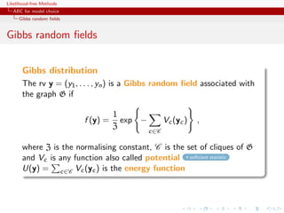
For Gibbs random fields , existence of a genuine sufficient statistic η(y).
[Møller, Pettitt, Berthelsen, Reeves, 2006]](https://image.slidesharecdn.com/romabc-120120013357-phpapp02/85/ABC-in-Roma-234-320.jpg)
![Likelihood-free Methods
Approximate Bayesian computation
Automated summary statistic selection
Auxiliary variables and ABC
Special case of ABC when
g (z|θ, y) = K (η(bz) − η(y))
˜ ˜ ˜ ˜
f (y|θ )f (z|θ)/f (y|θ)f (z |θ ) replaced by one [or not?!]](https://image.slidesharecdn.com/romabc-120120013357-phpapp02/85/ABC-in-Roma-235-320.jpg)
![Likelihood-free Methods
Approximate Bayesian computation
Automated summary statistic selection
Auxiliary variables and ABC
Special case of ABC when
g (z|θ, y) = K (η(bz) − η(y))
˜ ˜ ˜ ˜
f (y|θ )f (z|θ)/f (y|θ)f (z |θ ) replaced by one [or not?!]
Consequences
likelihood-free (ABC) versus constant-free (AVM)
in ABC, K (·) should be allowed to depend on θ
for Gibbs random fields, the auxiliary approach should be
prefered to ABC
[Møller, 2012]](https://image.slidesharecdn.com/romabc-120120013357-phpapp02/85/ABC-in-Roma-236-320.jpg)
![Likelihood-free Methods
Approximate Bayesian computation
Automated summary statistic selection
ABC and BIC
Idea of applying BIC during the local regression :
Run regular ABC
Select summary statistics during local regression
Recycle the prior simulation sample (reference table) with
those summary statistics
Rerun the corresponding local regression (low cost)
[Pudlo Sedki, 2012]](https://image.slidesharecdn.com/romabc-120120013357-phpapp02/85/ABC-in-Roma-237-320.jpg)


![Likelihood-free Methods
ABC for model choice
Model choice
ABC estimates
Posterior probability π(M = m|y) approximated by the frequency
of acceptances from model m
T
1
Im(t) =m .
T
t=1
Extension to a weighted polychotomous logistic regression estimate
of π(M = m|y), with non-parametric kernel weights
[Cornuet et al., DIYABC, 2009]](https://image.slidesharecdn.com/romabc-120120013357-phpapp02/85/ABC-in-Roma-243-320.jpg)

![Likelihood-free Methods
ABC for model choice
Model choice
The Great ABC controversy
On-going controvery in phylogeographic genetics about the validity
of using ABC for testing
Replies: Fagundes et al., 2008,
Against: Templeton, 2008, Beaumont et al., 2010, Berger et
2009, 2010a, 2010b, 2010c al., 2010, Csill`ry et al., 2010
e
argues that nested hypotheses point out that the criticisms are
cannot have higher probabilities addressed at [Bayesian]
than nesting hypotheses (!) model-based inference and have
nothing to do with ABC...](https://image.slidesharecdn.com/romabc-120120013357-phpapp02/85/ABC-in-Roma-245-320.jpg)


![Likelihood-free Methods
ABC for model choice
Gibbs random fields
Potts model
Potts model
Vc (y) is of the form
Vc (y) = θS(y) = θ δyl =yi
l∼i
where l∼i denotes a neighbourhood structure
In most realistic settings, summation
Zθ = exp{θ T S(x)}
x∈X
involves too many terms to be manageable and numerical
approximations cannot always be trusted
[Cucala, Marin, CPR Titterington, 2009]](https://image.slidesharecdn.com/romabc-120120013357-phpapp02/85/ABC-in-Roma-249-320.jpg)


![Likelihood-free Methods
ABC for model choice
Gibbs random fields
Sufficient statistics in Gibbs random fields
For Gibbs random fields,
1 2
x|M = m ∼ fm (x|θm ) = fm (x|S(x))fm (S(x)|θm )
1
= f 2 (S(x)|θm )
n(S(x)) m
where
n(S(x)) = {˜ ∈ X : S(˜) = S(x)}
x x
c S(x) is therefore also sufficient for the joint parameters
[Specific to Gibbs random fields!]](https://image.slidesharecdn.com/romabc-120120013357-phpapp02/85/ABC-in-Roma-257-320.jpg)


![Likelihood-free Methods
ABC for model choice
Generic ABC model choice
Back to sufficiency
‘Sufficient statistics for individual models are unlikely to
be very informative for the model probability.’
[Scott Sisson, Jan. 31, 2011, X.’Og]](https://image.slidesharecdn.com/romabc-120120013357-phpapp02/85/ABC-in-Roma-263-320.jpg)
![Likelihood-free Methods
ABC for model choice
Generic ABC model choice
Back to sufficiency
‘Sufficient statistics for individual models are unlikely to
be very informative for the model probability.’
[Scott Sisson, Jan. 31, 2011, X.’Og]
If η1 (x) sufficient statistic for model m = 1 and parameter θ1 and
η2 (x) sufficient statistic for model m = 2 and parameter θ2 ,
(η1 (x), η2 (x)) is not always sufficient for (m, θm )](https://image.slidesharecdn.com/romabc-120120013357-phpapp02/85/ABC-in-Roma-264-320.jpg)
![Likelihood-free Methods
ABC for model choice
Generic ABC model choice
Back to sufficiency
‘Sufficient statistics for individual models are unlikely to
be very informative for the model probability.’
[Scott Sisson, Jan. 31, 2011, X.’Og]
If η1 (x) sufficient statistic for model m = 1 and parameter θ1 and
η2 (x) sufficient statistic for model m = 2 and parameter θ2 ,
(η1 (x), η2 (x)) is not always sufficient for (m, θm )
c Potential loss of information at the testing level](https://image.slidesharecdn.com/romabc-120120013357-phpapp02/85/ABC-in-Roma-265-320.jpg)


![Likelihood-free Methods
ABC for model choice
Generic ABC model choice
Limiting behaviour of B12 (under sufficiency)
If η(y) sufficient statistic for both models,
fi (y|θ i ) = gi (y)fi η (η(y)|θ i )
Thus
Θ1 π(θ 1 )g1 (y)f1η (η(y)|θ 1 ) dθ 1
B12 (y) =
Θ2 π(θ 2 )g2 (y)f2η (η(y)|θ 2 ) dθ 2
g1 (y) π1 (θ 1 )f1η (η(y)|θ 1 ) dθ 1 g1 (y) η
= η = B (y) .
g2 (y) π2 (θ 2 )f2 (η(y)|θ 2 ) dθ 2 g2 (y) 12
[Didelot, Everitt, Johansen Lawson, 2011]](https://image.slidesharecdn.com/romabc-120120013357-phpapp02/85/ABC-in-Roma-270-320.jpg)
![Likelihood-free Methods
ABC for model choice
Generic ABC model choice
Limiting behaviour of B12 (under sufficiency)
If η(y) sufficient statistic for both models,
fi (y|θ i ) = gi (y)fi η (η(y)|θ i )
Thus
Θ1 π(θ 1 )g1 (y)f1η (η(y)|θ 1 ) dθ 1
B12 (y) =
Θ2 π(θ 2 )g2 (y)f2η (η(y)|θ 2 ) dθ 2
g1 (y) π1 (θ 1 )f1η (η(y)|θ 1 ) dθ 1 g1 (y) η
= η = B (y) .
g2 (y) π2 (θ 2 )f2 (η(y)|θ 2 ) dθ 2 g2 (y) 12
[Didelot, Everitt, Johansen Lawson, 2011]
c No discrepancy only when cross-model sufficiency](https://image.slidesharecdn.com/romabc-120120013357-phpapp02/85/ABC-in-Roma-271-320.jpg)


![Likelihood-free Methods
ABC for model choice
Generic ABC model choice
Formal recovery
Creating an encompassing exponential family
T T
f (x|θ1 , θ2 , α1 , α2 ) ∝ exp{θ1 η1 (x) + θ1 η1 (x) + α1 t1 (x) + α2 t2 (x)}
leads to a sufficient statistic (η1 (x), η2 (x), t1 (x), t2 (x))
[Didelot, Everitt, Johansen Lawson, 2011]](https://image.slidesharecdn.com/romabc-120120013357-phpapp02/85/ABC-in-Roma-274-320.jpg)
![Likelihood-free Methods
ABC for model choice
Generic ABC model choice
Formal recovery
Creating an encompassing exponential family
T T
f (x|θ1 , θ2 , α1 , α2 ) ∝ exp{θ1 η1 (x) + θ1 η1 (x) + α1 t1 (x) + α2 t2 (x)}
leads to a sufficient statistic (η1 (x), η2 (x), t1 (x), t2 (x))
[Didelot, Everitt, Johansen Lawson, 2011]
In the Poisson/geometric case, if i xi ! is added to S, no
discrepancy](https://image.slidesharecdn.com/romabc-120120013357-phpapp02/85/ABC-in-Roma-275-320.jpg)
![Likelihood-free Methods
ABC for model choice
Generic ABC model choice
Formal recovery
Creating an encompassing exponential family
T T
f (x|θ1 , θ2 , α1 , α2 ) ∝ exp{θ1 η1 (x) + θ1 η1 (x) + α1 t1 (x) + α2 t2 (x)}
leads to a sufficient statistic (η1 (x), η2 (x), t1 (x), t2 (x))
[Didelot, Everitt, Johansen Lawson, 2011]
Only applies in genuine sufficiency settings...
c Inability to evaluate loss brought by summary statistics](https://image.slidesharecdn.com/romabc-120120013357-phpapp02/85/ABC-in-Roma-276-320.jpg)
![Likelihood-free Methods
ABC for model choice
Generic ABC model choice
Meaning of the ABC-Bayes factor
‘This is also why focus on model discrimination typically
(...) proceeds by (...) accepting that the Bayes Factor
that one obtains is only derived from the summary
statistics and may in no way correspond to that of the
full model.’
[Scott Sisson, Jan. 31, 2011, X.’Og]](https://image.slidesharecdn.com/romabc-120120013357-phpapp02/85/ABC-in-Roma-277-320.jpg)
![Likelihood-free Methods
ABC for model choice
Generic ABC model choice
Meaning of the ABC-Bayes factor
‘This is also why focus on model discrimination typically
(...) proceeds by (...) accepting that the Bayes Factor
that one obtains is only derived from the summary
statistics and may in no way correspond to that of the
full model.’
[Scott Sisson, Jan. 31, 2011, X.’Og]
In the Poisson/geometric case, if E[yi ] = θ0 0,
η (θ0 + 1)2 −θ0
lim B12 (y) = e
n→∞ θ0](https://image.slidesharecdn.com/romabc-120120013357-phpapp02/85/ABC-in-Roma-278-320.jpg)
![Likelihood-free Methods
ABC for model choice
Generic ABC model choice
MA(q) divergence
0.7
0.6
0.6
0.6
0.6
0.5
0.5
0.5
0.5
0.4
0.4
0.4
0.4
0.3
0.3
0.3
0.3
0.2
0.2
0.2
0.2
0.1
0.1
0.1
0.1
0.0
0.0
0.0
0.0
1 2 1 2 1 2 1 2
Evolution [against ] of ABC Bayes factor, in terms of frequencies of
visits to models MA(1) (left) and MA(2) (right) when equal to
10, 1, .1, .01% quantiles on insufficient autocovariance distances. Sample
of 50 points from a MA(2) with θ1 = 0.6, θ2 = 0.2. True Bayes factor
equal to 17.71.](https://image.slidesharecdn.com/romabc-120120013357-phpapp02/85/ABC-in-Roma-279-320.jpg)
![Likelihood-free Methods
ABC for model choice
Generic ABC model choice
MA(q) divergence
0.8
0.6
0.6
0.6
0.6
0.4
0.4
0.4
0.4
0.2
0.2
0.2
0.2
0.0
0.0
0.0
0.0
1 2 1 2 1 2 1 2
Evolution [against ] of ABC Bayes factor, in terms of frequencies of
visits to models MA(1) (left) and MA(2) (right) when equal to
10, 1, .1, .01% quantiles on insufficient autocovariance distances. Sample
of 50 points from a MA(1) model with θ1 = 0.6. True Bayes factor B21
equal to .004.](https://image.slidesharecdn.com/romabc-120120013357-phpapp02/85/ABC-in-Roma-280-320.jpg)
![Likelihood-free Methods
ABC for model choice
Generic ABC model choice
Further comments
‘There should be the possibility that for the same model,
but different (non-minimal) [summary] statistics (so
∗
different η’s: η1 and η1 ) the ratio of evidences may no
longer be equal to one.’
[Michael Stumpf, Jan. 28, 2011, ’Og]
Using different summary statistics [on different models] may
indicate the loss of information brought by each set but agreement
does not lead to trustworthy approximations.](https://image.slidesharecdn.com/romabc-120120013357-phpapp02/85/ABC-in-Roma-281-320.jpg)

![Likelihood-free Methods
ABC for model choice
Generic ABC model choice
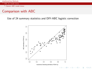
A population genetics evaluation
Population genetics example with
3 populations
2 scenari
15 individuals
5 loci
single mutation parameter
24 summary statistics
2 million ABC proposal
importance [tree] sampling alternative](https://image.slidesharecdn.com/romabc-120120013357-phpapp02/85/ABC-in-Roma-283-320.jpg)


![Likelihood-free Methods
ABC for model choice
Generic ABC model choice
The only safe cases???
Besides specific models like Gibbs random fields,
using distances over the data itself escapes the discrepancy...
[Toni Stumpf, 2010; Sousa al., 2009]](https://image.slidesharecdn.com/romabc-120120013357-phpapp02/85/ABC-in-Roma-288-320.jpg)
![Likelihood-free Methods
ABC for model choice
Generic ABC model choice
The only safe cases???
Besides specific models like Gibbs random fields,
using distances over the data itself escapes the discrepancy...
[Toni Stumpf, 2010; Sousa al., 2009]
...and so does the use of more informal model fitting measures
[Ratmann al., 2009]](https://image.slidesharecdn.com/romabc-120120013357-phpapp02/85/ABC-in-Roma-289-320.jpg)


![Likelihood-free Methods
ABC model choice consistency
Formalised framework
A benchmark if toy example
Comparison suggested by referee of PNAS paper [thanks]:
[X, Cornuet, Marin, Pillai, Aug. 2011]
Model M1 : y ∼ N (θ1 , 1) opposed to model M2 :
√
y ∼ L(θ2 , 1/ √ Laplace distribution with mean θ2 and scale
2),
parameter 1/ 2 (variance one).](https://image.slidesharecdn.com/romabc-120120013357-phpapp02/85/ABC-in-Roma-293-320.jpg)
![Likelihood-free Methods
ABC model choice consistency
Formalised framework
A benchmark if toy example
Comparison suggested by referee of PNAS paper [thanks]:
[X, Cornuet, Marin, Pillai, Aug. 2011]
Model M1 : y ∼ N (θ1 , 1) opposed to model M2 :
√
y ∼ L(θ2 , 1/ √ Laplace distribution with mean θ2 and scale
2),
parameter 1/ 2 (variance one).
Four possible statistics
1. sample mean y (sufficient for M1 if not M2 );
2. sample median med(y) (insufficient);
3. sample variance var(y) (ancillary);
4. median absolute deviation mad(y) = med(y − med(y));](https://image.slidesharecdn.com/romabc-120120013357-phpapp02/85/ABC-in-Roma-294-320.jpg)
![Likelihood-free Methods
ABC model choice consistency
Formalised framework
A benchmark if toy example
Comparison suggested by referee of PNAS paper [thanks]:
[X, Cornuet, Marin, Pillai, Aug. 2011]
Model M1 : y ∼ N (θ1 , 1) opposed to model M2 :
√
y ∼ L(θ2 , 1/ √ Laplace distribution with mean θ2 and scale
2),
parameter 1/ 2 (variance one).
6
5
4
Density
3
2
1
0
0.1 0.2 0.3 0.4 0.5 0.6 0.7
posterior probability](https://image.slidesharecdn.com/romabc-120120013357-phpapp02/85/ABC-in-Roma-295-320.jpg)
![Likelihood-free Methods
ABC model choice consistency
Formalised framework
A benchmark if toy example
Comparison suggested by referee of PNAS paper [thanks]:
[X, Cornuet, Marin, Pillai, Aug. 2011]
Model M1 : y ∼ N (θ1 , 1) opposed to model M2 :
√
y ∼ L(θ2 , 1/ √ Laplace distribution with mean θ2 and scale
2),
parameter 1/ 2 (variance one).
n=100
0.7
0.6
0.5
0.4
q
0.3
q
q
q
0.2
0.1
q
q
q
q
q
0.0
q
q
Gauss Laplace](https://image.slidesharecdn.com/romabc-120120013357-phpapp02/85/ABC-in-Roma-296-320.jpg)
![Likelihood-free Methods
ABC model choice consistency
Formalised framework
A benchmark if toy example
Comparison suggested by referee of PNAS paper [thanks]:
[X, Cornuet, Marin, Pillai, Aug. 2011]
Model M1 : y ∼ N (θ1 , 1) opposed to model M2 :
√
y ∼ L(θ2 , 1/ √ Laplace distribution with mean θ2 and scale
2),
parameter 1/ 2 (variance one).
6
3
5
4
Density
Density
2
3
2
1
1
0
0
0.1 0.2 0.3 0.4 0.5 0.6 0.7 0.0 0.2 0.4 0.6 0.8 1.0
posterior probability probability](https://image.slidesharecdn.com/romabc-120120013357-phpapp02/85/ABC-in-Roma-297-320.jpg)
![Likelihood-free Methods
ABC model choice consistency
Formalised framework
A benchmark if toy example
Comparison suggested by referee of PNAS paper [thanks]:
[X, Cornuet, Marin, Pillai, Aug. 2011]
Model M1 : y ∼ N (θ1 , 1) opposed to model M2 :
√
y ∼ L(θ2 , 1/ √ Laplace distribution with mean θ2 and scale
2),
parameter 1/ 2 (variance one).
n=100 n=100
1.0
0.7
q
q
0.6
q
0.8
q
q
0.5
q
q
q
0.6
q
0.4
q
q
q q
0.3
q
q
0.4
q
q
0.2
0.2
q
0.1
q
q
q q
q q
q
0.0
0.0
q
q
Gauss Laplace Gauss Laplace](https://image.slidesharecdn.com/romabc-120120013357-phpapp02/85/ABC-in-Roma-298-320.jpg)


![Likelihood-free Methods
ABC model choice consistency
Consistency results
Assumptions
A collection of asymptotic “standard” assumptions:
[A1] There exist a sequence {vn } converging to +∞,
an a.c. distribution Q with continuous bounded density q(·),
a symmetric, d × d positive definite matrix V0
and a vector µ0 ∈ Rd such that
−1/2 n→∞
vn V0 (Tn − µ0 ) Q, under Gn
and for all M 0
−d −1/2
sup |V0 |1/2 vn gn (t) − q vn V0 {t − µ0 } = o(1)
vn |t−µ0 |M](https://image.slidesharecdn.com/romabc-120120013357-phpapp02/85/ABC-in-Roma-301-320.jpg)
![Likelihood-free Methods
ABC model choice consistency
Consistency results
Assumptions
A collection of asymptotic “standard” assumptions:
[A2] For i = 1, 2, there exist d × d symmetric positive definite matrices
Vi (θi ) and µi (θi ) ∈ Rd such that
n→∞
vn Vi (θi )−1/2 (Tn − µi (θi )) Q, under Gi,n (·|θi ) .](https://image.slidesharecdn.com/romabc-120120013357-phpapp02/85/ABC-in-Roma-302-320.jpg)
![Likelihood-free Methods
ABC model choice consistency
Consistency results
Assumptions
A collection of asymptotic “standard” assumptions:
[A3] For i = 1, 2, there exist sets Fn,i ⊂ Θi and constants i , τi , αi 0
such that for all τ 0,
sup Gi,n |Tn − µ(θi )| τ |µi (θi ) − µ0 | ∧ i |θi
θi ∈Fn,i
−α −αi
vn i sup (|µi (θi ) − µ0 | ∧ i )
θi ∈Fn,i
with
c −τ
πi (Fn,i ) = o(vn i ).](https://image.slidesharecdn.com/romabc-120120013357-phpapp02/85/ABC-in-Roma-303-320.jpg)
![Likelihood-free Methods
ABC model choice consistency
Consistency results
Assumptions
A collection of asymptotic “standard” assumptions:
[A4] For u 0
−1
Sn,i (u) = θi ∈ Fn,i ; |µ(θi ) − µ0 | ≤ u vn
if inf{|µi (θi ) − µ0 |; θi ∈ Θi } = 0, there exist constants di τi ∧ αi − 1
such that
−d
πi (Sn,i (u)) ∼ u di vn i , ∀u vn](https://image.slidesharecdn.com/romabc-120120013357-phpapp02/85/ABC-in-Roma-304-320.jpg)
![Likelihood-free Methods
ABC model choice consistency
Consistency results
Assumptions
A collection of asymptotic “standard” assumptions:
[A5] If inf{|µi (θi ) − µ0 |; θi ∈ Θi } = 0, there exists U 0 such that for
any M 0,
−d
sup sup |Vi (θi )|1/2 vn gi (t|θi )
vn |t−µ0 |M θi ∈Sn,i (U)
−q vn Vi (θi )−1/2 (t − µ(θi ) = o(1)
and
πi Sn,i (U) ∩ ||Vi (θi )−1 || + ||Vi (θi )|| M
lim lim sup =0.
M→∞ n πi (Sn,i (U))](https://image.slidesharecdn.com/romabc-120120013357-phpapp02/85/ABC-in-Roma-305-320.jpg)
![Likelihood-free Methods
ABC model choice consistency
Consistency results
Assumptions
A collection of asymptotic “standard” assumptions:
[A1]–[A2] are standard central limit theorems ([A1] redundant
when one model is “true”)
[A3] controls the large deviations of the estimator Tn from the
estimand µ(θ)
[A4] is the standard prior mass condition found in Bayesian
asymptotics (di effective dimension of the parameter)
[A5] controls more tightly convergence esp. when µi is not
one-to-one](https://image.slidesharecdn.com/romabc-120120013357-phpapp02/85/ABC-in-Roma-306-320.jpg)
![Likelihood-free Methods
ABC model choice consistency
Consistency results
Effective dimension
[A4] Understanding d1 , d2 : defined only when
µ0 ∈ {µi (θi ), θi ∈ Θi },
πi (θi : |µi (θi ) − µ0 | n−1/2 ) = O(n−di /2 )
is the effective dimension of the model Θi around µ0](https://image.slidesharecdn.com/romabc-120120013357-phpapp02/85/ABC-in-Roma-307-320.jpg)
![Likelihood-free Methods
ABC model choice consistency
Consistency results
Asymptotic marginals
Asymptotically, under [A1]–[A5]
mi (t) = gi (t|θi ) πi (θi ) dθi
Θi
is such that
(i) if inf{|µi (θi ) − µ0 |; θi ∈ Θi } = 0,
Cl vn i ≤ mi (Tn ) ≤ Cu vn i
d−d d−d
and
(ii) if inf{|µi (θi ) − µ0 |; θi ∈ Θi } 0
mi (Tn ) = oPn [vn i + vn i ].
d−τ d−α](https://image.slidesharecdn.com/romabc-120120013357-phpapp02/85/ABC-in-Roma-308-320.jpg)


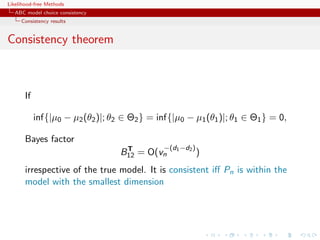


![Likelihood-free Methods
ABC model choice consistency
Summary statistics
Toy example: Laplace versus Gauss [1]
If
n
Tn = n−1 Xi4 , µ1 (θ) = 3 + θ4 + 6θ2 , µ2 (θ) = 6 + · · ·
i=1
and the true distribution is Laplace with mean θ0 = 1, under the
√
Gaussian model the value θ∗ = 2 3 − 3 leads to µ0 = µ(θ∗ )
[here d1 = d2 = d = 1]](https://image.slidesharecdn.com/romabc-120120013357-phpapp02/85/ABC-in-Roma-317-320.jpg)
![Likelihood-free Methods
ABC model choice consistency
Summary statistics
Toy example: Laplace versus Gauss [1]
If
n
Tn = n−1 Xi4 , µ1 (θ) = 3 + θ4 + 6θ2 , µ2 (θ) = 6 + · · ·
i=1
and the true distribution is Laplace with mean θ0 = 1, under the
√
Gaussian model the value θ∗ = 2 3 − 3 leads to µ0 = µ(θ∗ )
[here d1 = d2 = d = 1]
c a Bayes factor associated with such a statistic is inconsistent](https://image.slidesharecdn.com/romabc-120120013357-phpapp02/85/ABC-in-Roma-318-320.jpg)
![Likelihood-free Methods
ABC model choice consistency
Summary statistics
Toy example: Laplace versus Gauss [1]
If
n
n −1
T =n Xi4 , µ1 (θ) = 3 + θ4 + 6θ2 , µ2 (θ) = 6 + · · ·
i=1
8
6
4
2
0
0.0 0.2 0.4 0.6 0.8 1.0
probability
Fourth moment](https://image.slidesharecdn.com/romabc-120120013357-phpapp02/85/ABC-in-Roma-319-320.jpg)
![Likelihood-free Methods
ABC model choice consistency
Summary statistics
Toy example: Laplace versus Gauss [1]
If
n
n −1
T =n Xi4 , µ1 (θ) = 3 + θ4 + 6θ2 , µ2 (θ) = 6 + · · ·
i=1
n=1000
0.45
q
0.40
0.35
q
q
q
0.30
q
M1 M2](https://image.slidesharecdn.com/romabc-120120013357-phpapp02/85/ABC-in-Roma-320-320.jpg)
![Likelihood-free Methods
ABC model choice consistency
Summary statistics
Toy example: Laplace versus Gauss [1]
If
n
n −1
T =n Xi4 , µ1 (θ) = 3 + θ4 + 6θ2 , µ2 (θ) = 6 + · · ·
i=1
Caption: Comparison of the distributions of the posterior
probabilities that the data is from a normal model (as opposed to a
Laplace model) with unknown mean when the data is made of
n = 1000 observations either from a normal (M1) or Laplace (M2)
distribution with mean one and when the summary statistic in the
ABC algorithm is restricted to the empirical fourth moment. The
ABC algorithm uses proposals from the prior N (0, 4) and selects
the tolerance as the 1% distance quantile.](https://image.slidesharecdn.com/romabc-120120013357-phpapp02/85/ABC-in-Roma-321-320.jpg)
![Likelihood-free Methods
ABC model choice consistency
Summary statistics
Toy example: Laplace versus Gauss [0]
When
(4) (6)
T(y) = yn , yn
¯ ¯
and the true distribution is Laplace with mean θ0 = 0, then
√
∗ ∗
µ0 = 6, µ1 (θ1 ) = 6 with θ1 = 2 3 − 3
[d1 = 1 and d2 = 1/2]
thus
B12 ∼ n−1/4 → 0 : consistent](https://image.slidesharecdn.com/romabc-120120013357-phpapp02/85/ABC-in-Roma-322-320.jpg)
![Likelihood-free Methods
ABC model choice consistency
Summary statistics
Toy example: Laplace versus Gauss [0]
When
(4) (6)
T(y) = yn , yn
¯ ¯
and the true distribution is Laplace with mean θ0 = 0, then
√
∗ ∗
µ0 = 6, µ1 (θ1 ) = 6 with θ1 = 2 3 − 3
[d1 = 1 and d2 = 1/2]
thus
B12 ∼ n−1/4 → 0 : consistent
Under the Gaussian model µ0 = 3 µ2 (θ2 ) ≥ 6 3 ∀θ2
B12 → +∞ : consistent](https://image.slidesharecdn.com/romabc-120120013357-phpapp02/85/ABC-in-Roma-323-320.jpg)
![Likelihood-free Methods
ABC model choice consistency
Summary statistics
Toy example: Laplace versus Gauss [0]
When
(4) (6)
T(y) = yn , yn
¯ ¯
5
4
3
Density
2
1
0
0.0 0.2 0.4 0.6 0.8 1.0
posterior probabilities
Fourth and sixth moments](https://image.slidesharecdn.com/romabc-120120013357-phpapp02/85/ABC-in-Roma-324-320.jpg)


Likelihood-free methods provide techniques for approximating Bayesian computations when the likelihood function is unavailable or computationally intractable. Monte Carlo methods like importance sampling and iterated importance sampling generate samples from an approximating distribution to estimate integrals. Population Monte Carlo is an iterative Monte Carlo algorithm that propagates a population of particles over time to explore the target distribution. Approximate Bayesian computation uses simulation-based methods to approximate posterior distributions when the likelihood is unavailable.